

Image Change Detection and Fusion Using MRF Models
287
is 4096 x 4096 for an image of size (64 x 64) pixels). The suboptimum approach
of considering one sub image at a time sacrifices optimality for computational
efficiency. However, the statistical correlation among sites is concentrated
in regions that are only a few sites apart. Therefore, our approximation is
reasonable and yields satisfactory results in the examples.
The optimal algorithm used here involves matrix inversion and multiplication, both of which have the computational complexity O(n 3 ) for an image
of size n x n. During each iteration, Lb given in (12.23), is computed at least
2n2 times. As a result, the total complexity of our optimal algorithm is O(n 5 ).
However, when we employ the suboptimum algorithm, the number of operations for each subimage is fixed. Consequently, the overall complexity reduces
to O(n2).
12.3.1
Example 1: Synthetic Data
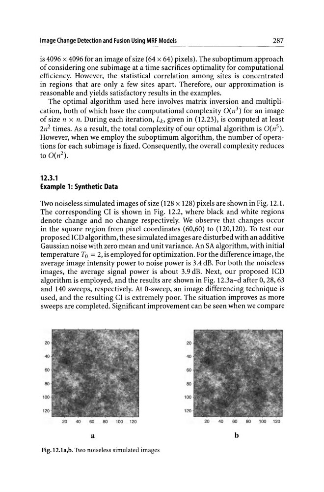
Two noiseless simulated images of size (128 x 128) pixels are shown in Fig. 12.1.
The corresponding CI is shown in Fig. 12.2, where black and white regions
denote change and no change respectively. We observe that changes occur
in the square region from pixel coordinates (60,60) to (120,120). To test our
proposed ICD algorithm, these simulated images are disturbed with an additive
Gaussian noise with zero mean and unit variance. An SA algorithm, with initial
temperature To = 2, is employed for optimization. For the difference image, the
average image intensity power to noise power is 3.4 dB. For both the noiseless
images, the average signal power is about 3.9 dB. Next, our proposed ICD
algorithm is employed, and the results are shown in Fig. 12.3a-d after 0, 28, 63
and 140 sweeps, respectively. At O-sweep, an image differencing technique is
used, and the resulting CI is extremely poor. The situation improves as more
sweeps are completed. Significant improvement can be seen when we compare
20
40
60
80
100
120
120
20
40
60
80
100 120
20
40
60
80
100
120
a
b
Fig.12.1a,b. Two noiseless simulated images
287
is 4096 x 4096 for an image of size (64 x 64) pixels). The suboptimum approach
of considering one sub image at a time sacrifices optimality for computational
efficiency. However, the statistical correlation among sites is concentrated
in regions that are only a few sites apart. Therefore, our approximation is
reasonable and yields satisfactory results in the examples.
The optimal algorithm used here involves matrix inversion and multiplication, both of which have the computational complexity O(n 3 ) for an image
of size n x n. During each iteration, Lb given in (12.23), is computed at least
2n2 times. As a result, the total complexity of our optimal algorithm is O(n 5 ).
However, when we employ the suboptimum algorithm, the number of operations for each subimage is fixed. Consequently, the overall complexity reduces
to O(n2).
12.3.1
Example 1: Synthetic Data
Two noiseless simulated images of size (128 x 128) pixels are shown in Fig. 12.1.
The corresponding CI is shown in Fig. 12.2, where black and white regions
denote change and no change respectively. We observe that changes occur
in the square region from pixel coordinates (60,60) to (120,120). To test our
proposed ICD algorithm, these simulated images are disturbed with an additive
Gaussian noise with zero mean and unit variance. An SA algorithm, with initial
temperature To = 2, is employed for optimization. For the difference image, the
average image intensity power to noise power is 3.4 dB. For both the noiseless
images, the average signal power is about 3.9 dB. Next, our proposed ICD
algorithm is employed, and the results are shown in Fig. 12.3a-d after 0, 28, 63
and 140 sweeps, respectively. At O-sweep, an image differencing technique is
used, and the resulting CI is extremely poor. The situation improves as more
sweeps are completed. Significant improvement can be seen when we compare
20
40
60
80
100
120
120
20
40
60
80
100 120
20
40
60
80
100
120
a
b
Fig.12.1a,b. Two noiseless simulated images