

Image Change Detection and Fusion Using MRF Models
285
where P(y Ix) and P(Xi,xj IHI) denote P(Y = Y IX = x), and P(Xi = Xi,Xj =
Xj IHI), respectively.
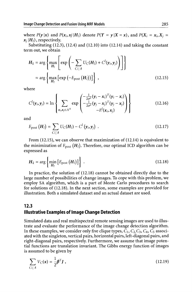
Substituting (12.3), (12.4) and (12.lO) into (12.14) and taking the constant
term out, we obtain
Hk = .,g h~ [exp ( -~ Uc(HJ) + C(y;, Yj») ] I
= arg {~~ [exp (-Epost{HI))]} ,
(12.15)
where
(12.16)
and
Epost (HI) = L UdHI) - d (yi,Yj)
(12.17)
Cc-S
From (12.15), we can observe that maximization of (12.14) is equivalent to
the minimization of Epost (HI). Therefore, our optimal ICD algorithm can be
expressed as
Hk = arg {rw[n [Epost (HI)]} .
(12.18)
In practice, the solution of (12.18) cannot be obtained directly due to the
large number of possibilities of change images. To cope with this problem, we
employ SA algorithm, which is a part of Monte Carlo procedures to search
for solutions of (12.18). In the next section, some examples are provided for
illustration. Both a simulated dataset and an actual dataset are used.
12.3
Illustrative Examples of Image Change Detection
Simulated data and real multispectral remote sensing images are used to illustrate and evaluate the performance of the image change detection algorithm.
In these examples, we consider only five clique types, C1, C2, C3, C4, Cs associated with the singleton, vertical pairs, horizontal pairs, left-diagonal pairs, and
right-diagonal pairs, respectively. Furthermore, we assume that image potential functions are translation invariant. The Gibbs energy function of images
is assumed to be given by
(12.19)
285
where P(y Ix) and P(Xi,xj IHI) denote P(Y = Y IX = x), and P(Xi = Xi,Xj =
Xj IHI), respectively.
Substituting (12.3), (12.4) and (12.lO) into (12.14) and taking the constant
term out, we obtain
Hk = .,g h~ [exp ( -~ Uc(HJ) + C(y;, Yj») ] I
= arg {~~ [exp (-Epost{HI))]} ,
(12.15)
where
(12.16)
and
Epost (HI) = L UdHI) - d (yi,Yj)
(12.17)
Cc-S
From (12.15), we can observe that maximization of (12.14) is equivalent to
the minimization of Epost (HI). Therefore, our optimal ICD algorithm can be
expressed as
Hk = arg {rw[n [Epost (HI)]} .
(12.18)
In practice, the solution of (12.18) cannot be obtained directly due to the
large number of possibilities of change images. To cope with this problem, we
employ SA algorithm, which is a part of Monte Carlo procedures to search
for solutions of (12.18). In the next section, some examples are provided for
illustration. Both a simulated dataset and an actual dataset are used.
12.3
Illustrative Examples of Image Change Detection
Simulated data and real multispectral remote sensing images are used to illustrate and evaluate the performance of the image change detection algorithm.
In these examples, we consider only five clique types, C1, C2, C3, C4, Cs associated with the singleton, vertical pairs, horizontal pairs, left-diagonal pairs, and
right-diagonal pairs, respectively. Furthermore, we assume that image potential functions are translation invariant. The Gibbs energy function of images
is assumed to be given by
(12.19)