

272
11: Teerasit Kasetkasem, Manoj K. Arora, Pramod K. Varshney
Component 1
20
20
40
40
60
60
20
40
60
80
100 120
20
40
60
80
100 120
Component 3
20
20
40
40
60
60
20
40
60
80
100 120
20
40
60
80
100 120
ComponentS
Component 6
20
20
40
40
60
60
20
40
60
80
100 120
20
40
60
80
100 120
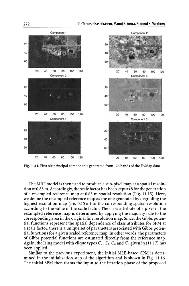
Fig.ll.ll. First six principal components generated from 126 bands of the HyMap data
The MRF model is then used to produce a sub-pixel map at a spatial resolution of 0.85 m. Accordingly, the scale factor has been kept as 8 for the generation
of a resampled reference map at 0.85 m spatial resolution (Fig. 11.15). Here,
we define the resampled reference map as the one generated by degrading the
highest resolution map (i. e. 0.15 m) to the corresponding spatial resolution
according to the value of the scale factor. The class attribute of a pixel in the
resampled reference map is determined by applying the majority rule to the
corresponding area in the original fine resolution map. Since, the Gibbs potential functions represent the spatial dependence of class attributes for SPM at
a scale factor, there is a unique set of parameters associated with Gibbs potential functions for a given scaled reference map. In other words, the parameters
of Gibbs potential functions are estimated directly from the reference map.
Again, the Ising model with clique types C2, C3, C4 and Cs given in (i1.1?) has
been applied.
Similar to the previous experiment, the initial MLE-based SPM is determined in the initialization step of the algorithm and is shown in Fig. 11.16.
The initial SPM then forms the input to the iteration phase of the proposed
11: Teerasit Kasetkasem, Manoj K. Arora, Pramod K. Varshney
Component 1
20
20
40
40
60
60
20
40
60
80
100 120
20
40
60
80
100 120
Component 3
20
20
40
40
60
60
20
40
60
80
100 120
20
40
60
80
100 120
ComponentS
Component 6
20
20
40
40
60
60
20
40
60
80
100 120
20
40
60
80
100 120
Fig.ll.ll. First six principal components generated from 126 bands of the HyMap data
The MRF model is then used to produce a sub-pixel map at a spatial resolution of 0.85 m. Accordingly, the scale factor has been kept as 8 for the generation
of a resampled reference map at 0.85 m spatial resolution (Fig. 11.15). Here,
we define the resampled reference map as the one generated by degrading the
highest resolution map (i. e. 0.15 m) to the corresponding spatial resolution
according to the value of the scale factor. The class attribute of a pixel in the
resampled reference map is determined by applying the majority rule to the
corresponding area in the original fine resolution map. Since, the Gibbs potential functions represent the spatial dependence of class attributes for SPM at
a scale factor, there is a unique set of parameters associated with Gibbs potential functions for a given scaled reference map. In other words, the parameters
of Gibbs potential functions are estimated directly from the reference map.
Again, the Ising model with clique types C2, C3, C4 and Cs given in (i1.1?) has
been applied.
Similar to the previous experiment, the initial MLE-based SPM is determined in the initialization step of the algorithm and is shown in Fig. 11.16.
The initial SPM then forms the input to the iteration phase of the proposed