

268
11: Teerasit Kasetkasem, Manoj K. Arora, Pramod K. Varshney
Due to the availability of the crisp reference image of the SPM, the MPLE
algorithm is employed for estimation of the parameters of the Gibbs potential function. The MPLE algorithm selects the sets of Gibbs parameters that
maximize the product of all the local characteristic functions of X( J), i. e.,
PMPlE = acg [ mr (!J P, (X(,) IX(N,) »)] .
(1Ll8)
Here, for the four clique types, the associated parameters, /32, /33, /34 and /35 are
obtained as 1.1, Ll, 0.3 and 0.3, respectively. However, if the crisp reference
image is not available, we can choose some appropriate values for /3 such as
fJ = [1 1 1 1] to make the SPM smooth (or having more connected regions). It
is obvious that this approach is quite heuristic, but it is based on the common
knowledge that a land cover map is generally composed of connected regions
rather than isolated points.
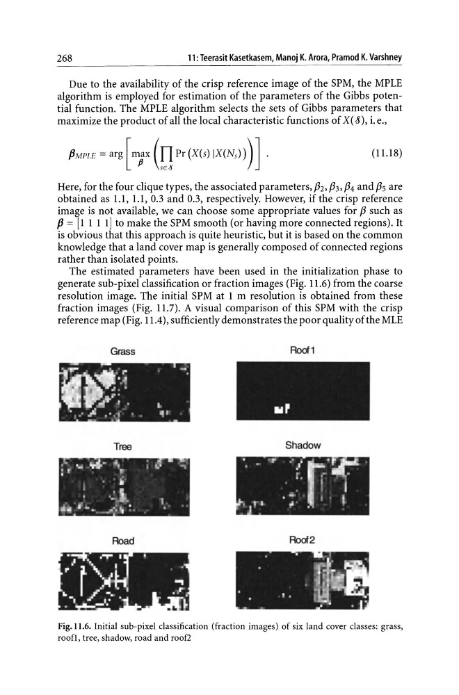
The estimated parameters have been used in the initialization phase to
generate sub-pixel classification or fraction images (Fig. 11.6) from the coarse
resolution image. The initial SPM at 1 m resolution is obtained from these
fraction images (Fig. 11.7). A visual comparison of this SPM with the crisp
reference map (Fig. 1104), sufficiently demonstrates the poor quality of the MLE
Grass
Rod 1
. . " . . *. -
•
0
r
0
'.of
J . •
~.r; 0
I
• ,.0 JI! 0':"
' "
Tree
Shadow
o . : -r.,4.. .., ; I. ...
: I
r
. ,
: .~ 1.
I
.b i - . J"':" :
•
' . • ' r
oo{r' ~
.
I
•
• I
• ;
I
,
.
Road
Rod 2
. .~. .
r" to .. , ·
0
.....
. ' . ,
~
I..
,
-....
• •
,
•
,.
L
•
: - - .
I
r
Fig. 1 1.6. Initial sub-pixel classification (fraction images) of six land cover classes: grass,
roofl, tree, shadow, road and roof2
11: Teerasit Kasetkasem, Manoj K. Arora, Pramod K. Varshney
Due to the availability of the crisp reference image of the SPM, the MPLE
algorithm is employed for estimation of the parameters of the Gibbs potential function. The MPLE algorithm selects the sets of Gibbs parameters that
maximize the product of all the local characteristic functions of X( J), i. e.,
PMPlE = acg [ mr (!J P, (X(,) IX(N,) »)] .
(1Ll8)
Here, for the four clique types, the associated parameters, /32, /33, /34 and /35 are
obtained as 1.1, Ll, 0.3 and 0.3, respectively. However, if the crisp reference
image is not available, we can choose some appropriate values for /3 such as
fJ = [1 1 1 1] to make the SPM smooth (or having more connected regions). It
is obvious that this approach is quite heuristic, but it is based on the common
knowledge that a land cover map is generally composed of connected regions
rather than isolated points.
The estimated parameters have been used in the initialization phase to
generate sub-pixel classification or fraction images (Fig. 11.6) from the coarse
resolution image. The initial SPM at 1 m resolution is obtained from these
fraction images (Fig. 11.7). A visual comparison of this SPM with the crisp
reference map (Fig. 1104), sufficiently demonstrates the poor quality of the MLE
Grass
Rod 1
. . " . . *. -
•
0
r
0
'.of
J . •
~.r; 0
I
• ,.0 JI! 0':"
' "
Tree
Shadow
o . : -r.,4.. .., ; I. ...
: I
r
. ,
: .~ 1.
I
.b i - . J"':" :
•
' . • ' r
oo{r' ~
.
I
•
• I
• ;
I
,
.
Road
Rod 2
. .~. .
r" to .. , ·
0
.....
. ' . ,
~
I..
,
-....
• •
,
•
,.
L
•
: - - .
I
r
Fig. 1 1.6. Initial sub-pixel classification (fraction images) of six land cover classes: grass,
roofl, tree, shadow, road and roof2