

262
11: Teerasit Kasetkasem, Manoj K. Arora, Pramod K. Varshney
where C = Z(2!)K/2' and
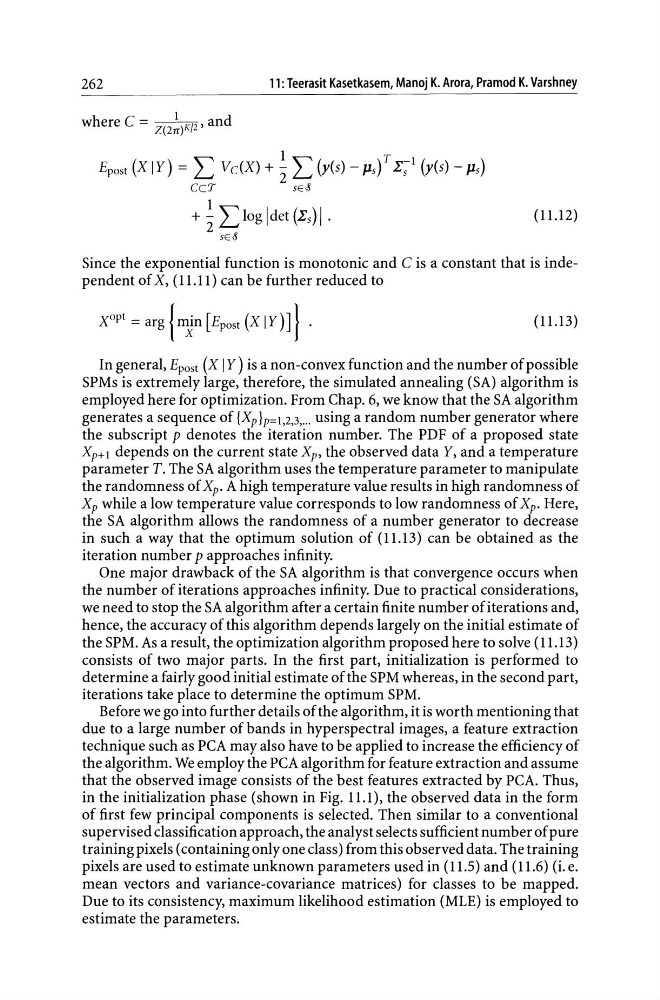
Epost (XIY) = L VdX) + ~ L (y(s) - Jls)T I;l (y(s) - Jls)
CeT
SE-8
1
+"2 Llog Idet (Is)l·
SE-8
(1Ll2)
Since the exponential function is monotonic and C is a constant that is independent of X, (1Ll1) can be further reduced to
Xopt = arg {mjn [Epost (X IY)]} .
(1Ll3)
In general, Epost (X I Y) is a non-convex function and the number of possible
SPMs is extremely large, therefore, the simulated annealing (SA) algorithm is
employed here for optimization. From Chap. 6, we know that the SA algorithm
generates a sequence of {Xp}p=1,2,3,,,. using a random number generator where
the subscript p denotes the iteration number. The PDF of a proposed state
Xp+l depends on the current state Xp, the observed data Y, and a temperature
parameter T. The SA algorithm uses the temperature parameter to manipulate
the randomness of Xp. A high temperature value results in high randomness of
Xp while a low temperature value corresponds to low randomness of Xp. Here,
the SA algorithm allows the randomness of a number generator to decrease
in such a way that the optimum solution of (1Ll3) can be obtained as the
iteration number p approaches infinity.
One major drawback of the SA algorithm is that convergence occurs when
the number of iterations approaches infinity. Due to practical considerations,
we need to stop the SA algorithm after a certain finite number of iterations and,
hence, the accuracy of this algorithm depends largely on the initial estimate of
the SPM. As a result, the optimization algorithm proposed here to solve (11.13)
consists of two major parts. In the first part, initialization is performed to
determine a fairly good initial estimate of the SPM whereas, in the second part,
iterations take place to determine the optimum SPM.
Before we go into further details of the algorithm, it is worth mentioning that
due to a large number of bands in hyperspectral images, a feature extraction
technique such as PCA may also have to be applied to increase the efficiency of
the algorithm. We employ the PCA algorithm for feature extraction and assume
that the observed image consists of the best features extracted by PCA. Thus,
in the initialization phase (shown in Fig. 11.1), the observed data in the form
of first few principal components is selected. Then similar to a conventional
supervised classification approach, the analyst selects sufficient number of pure
training pixels (containing only one class) from this observed data. The training
pixels are used to estimate unknown parameters used in (11.5) and (11.6) (i. e.
mean vectors and variance-covariance matrices) for classes to be mapped.
Due to its consistency, maximum likelihood estimation (MLE) is employed to
estimate the parameters.
11: Teerasit Kasetkasem, Manoj K. Arora, Pramod K. Varshney
where C = Z(2!)K/2' and
Epost (XIY) = L VdX) + ~ L (y(s) - Jls)T I;l (y(s) - Jls)
CeT
SE-8
1
+"2 Llog Idet (Is)l·
SE-8
(1Ll2)
Since the exponential function is monotonic and C is a constant that is independent of X, (1Ll1) can be further reduced to
Xopt = arg {mjn [Epost (X IY)]} .
(1Ll3)
In general, Epost (X I Y) is a non-convex function and the number of possible
SPMs is extremely large, therefore, the simulated annealing (SA) algorithm is
employed here for optimization. From Chap. 6, we know that the SA algorithm
generates a sequence of {Xp}p=1,2,3,,,. using a random number generator where
the subscript p denotes the iteration number. The PDF of a proposed state
Xp+l depends on the current state Xp, the observed data Y, and a temperature
parameter T. The SA algorithm uses the temperature parameter to manipulate
the randomness of Xp. A high temperature value results in high randomness of
Xp while a low temperature value corresponds to low randomness of Xp. Here,
the SA algorithm allows the randomness of a number generator to decrease
in such a way that the optimum solution of (1Ll3) can be obtained as the
iteration number p approaches infinity.
One major drawback of the SA algorithm is that convergence occurs when
the number of iterations approaches infinity. Due to practical considerations,
we need to stop the SA algorithm after a certain finite number of iterations and,
hence, the accuracy of this algorithm depends largely on the initial estimate of
the SPM. As a result, the optimization algorithm proposed here to solve (11.13)
consists of two major parts. In the first part, initialization is performed to
determine a fairly good initial estimate of the SPM whereas, in the second part,
iterations take place to determine the optimum SPM.
Before we go into further details of the algorithm, it is worth mentioning that
due to a large number of bands in hyperspectral images, a feature extraction
technique such as PCA may also have to be applied to increase the efficiency of
the algorithm. We employ the PCA algorithm for feature extraction and assume
that the observed image consists of the best features extracted by PCA. Thus,
in the initialization phase (shown in Fig. 11.1), the observed data in the form
of first few principal components is selected. Then similar to a conventional
supervised classification approach, the analyst selects sufficient number of pure
training pixels (containing only one class) from this observed data. The training
pixels are used to estimate unknown parameters used in (11.5) and (11.6) (i. e.
mean vectors and variance-covariance matrices) for classes to be mapped.
Due to its consistency, maximum likelihood estimation (MLE) is employed to
estimate the parameters.