

Markov Random Field Models
165
where L denotes the sum over those sets C that contain the site s. We write
C3S
Vc (A,X(.8\S)) to represent the Vdx') where x'(s) = A and x'(t) = x(t) for all
t E .8\s.
Theorem 6.1 has stated the first part of the relationship between MRFs and
Gibbs fields. We shall continue with the converse part, which will be formally
introduced in Theorem 6.2. Again, the proof of this theorem can be found in
Winkler (1995).
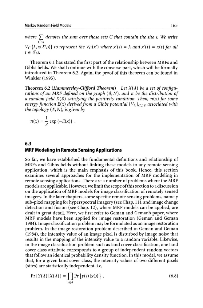
Theorem 6.2 (Hammersley-Clifford Theorem) Let X(.8) be a set of configurations of an MRF defined on the graph (.8, N), and 1£ be the distribution of
a random field X(.8) satisfying the positivity condition. Then, 1£(x) for some
energy function E(x) derived from a Gibbs potential {V c} CC -8 associated with
the topology ( .8, N), is given by
1
1£(x) = Z exp {-E(x)}
6.3
MRF Modeling in Remote Sensing Applications
So far, we have established the fundamental definitions and relationship of
MRFs and Gibbs fields without linking these models to any remote sensing
application, which is the main emphasis of this book. Hence, this section
examines several approaches for the implementation of MRF modeling in
remote sensing applications. There are a number of problems where the MRF
models are applicable. However, we limit the scope of this section to a discussion
on the application of MRF models for image classification of remotely sensed
imagery. In the later chapters, some specific remote sensing problems, namely
sub-pixel mapping for hyperspectral imagery (see Chap. 11), and image change
detection and fusion (see Chap. 12), where MRF models can be applied, are
dealt in great detail. Here, we first refer to Geman and Geman's paper, where
MRF models have been applied for image restoration (Geman and Geman
1984). Image classification problem may be formulated as an image restoration
problem. In the image restoration problem described in Geman and Geman
(1984), the intensity value of an image pixel is disturbed by image noise that
results in the mapping of the intensity value to a random variable. Likewise,
in the image classification problem such as land cover classification, one land
cover class attribute corresponds to a group of independent random vectors
that follow an identical probability density function. In this model, we assume
that, for a given land cover class, the intensity values of two different pixels
(sites) are statistically independent, i.e,
Pr {Y(.8) IX(.8) } = Tl Pr {y(s) Ix(s) } ,
(6.8)
SE-8
165
where L denotes the sum over those sets C that contain the site s. We write
C3S
Vc (A,X(.8\S)) to represent the Vdx') where x'(s) = A and x'(t) = x(t) for all
t E .8\s.
Theorem 6.1 has stated the first part of the relationship between MRFs and
Gibbs fields. We shall continue with the converse part, which will be formally
introduced in Theorem 6.2. Again, the proof of this theorem can be found in
Winkler (1995).
Theorem 6.2 (Hammersley-Clifford Theorem) Let X(.8) be a set of configurations of an MRF defined on the graph (.8, N), and 1£ be the distribution of
a random field X(.8) satisfying the positivity condition. Then, 1£(x) for some
energy function E(x) derived from a Gibbs potential {V c} CC -8 associated with
the topology ( .8, N), is given by
1
1£(x) = Z exp {-E(x)}
6.3
MRF Modeling in Remote Sensing Applications
So far, we have established the fundamental definitions and relationship of
MRFs and Gibbs fields without linking these models to any remote sensing
application, which is the main emphasis of this book. Hence, this section
examines several approaches for the implementation of MRF modeling in
remote sensing applications. There are a number of problems where the MRF
models are applicable. However, we limit the scope of this section to a discussion
on the application of MRF models for image classification of remotely sensed
imagery. In the later chapters, some specific remote sensing problems, namely
sub-pixel mapping for hyperspectral imagery (see Chap. 11), and image change
detection and fusion (see Chap. 12), where MRF models can be applied, are
dealt in great detail. Here, we first refer to Geman and Geman's paper, where
MRF models have been applied for image restoration (Geman and Geman
1984). Image classification problem may be formulated as an image restoration
problem. In the image restoration problem described in Geman and Geman
(1984), the intensity value of an image pixel is disturbed by image noise that
results in the mapping of the intensity value to a random variable. Likewise,
in the image classification problem such as land cover classification, one land
cover class attribute corresponds to a group of independent random vectors
that follow an identical probability density function. In this model, we assume
that, for a given land cover class, the intensity values of two different pixels
(sites) are statistically independent, i.e,
Pr {Y(.8) IX(.8) } = Tl Pr {y(s) Ix(s) } ,
(6.8)
SE-8