

166
6: Teerasit Kasetkasem
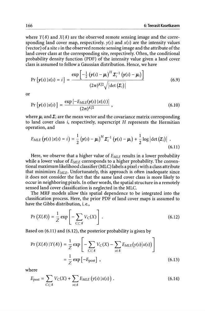
where Y(-8) and X(-8) are the observed remote sensing image and the corresponding land cover map, respectively. y(s) and x(s) are the intensity values
(vector) of a site s in the observed remote sensing image and the attribute of the
land cover class at the corresponding site, respectively. Often, the conditional
probability density function (PDF) of the intensity value given a land cover
class is assumed to follow a Gaussian distribution. Hence, we have
or
exp [-1 (y(s) - Pit IiI (y(s) - Pi)]
Pr {y(s) Ix(s) = i} = --=------,::===----=(2n)K/2 jldet (Ii) I
P { ( ) I ()} = exp [-EMLE(Y(S) Ix(s) )]
rys xs
K / 2 '
(2n)
(6.9)
(6.10)
where Pi andIi are the mean vector and the covariance matrix corresponding
to land cover class i, respectively, superscript H represents the Hermitian
operation, and
1
H
I I I
EMLE (y(s) Ix(s) = i) = - (y(s) - Pi) Ii (y(s) - Pi) + -log det (Ii) I .
2
2
(6.11)
Here, we observe that a higher value of EMLE results in a lower probability
while a lower value of EMLE corresponds to a higher probability. The conventional maximum likelihood classifier (MLC) labels a pixel s with a class attribute
that minimizes EMLE. Unfortunately, this approach is often inadequate since
it does not consider the fact that the same land cover class is more likely to
occur in neighboring pixels. In other words, the spatial structure in a remotely
sensed land cover classification is neglected in the MLC.
The MRF models allow this spatial dependence to be integrated into the
classification process. Here, the prior PDF of land cover maps is assumed to
have the Gibbs distribution, i. e.,
Pr (X(-8») = ~ exp [- L VdX )] .
Cc-8
Based on (6.11) and (6.12), the posterior probability is given by
Pr (X(-8) IY(-8») = ~ exp [- L VdX) - LEMLE(Y(s)lx(s»)]
Cc-8
SE-8
1
= Z exp [-Epost] ,
where
Epost = L VdX) + L EMLE (y(s) Ix(s») .
Cc-8
SE-8
(6.12)
(6.13)
(6.14)
6: Teerasit Kasetkasem
where Y(-8) and X(-8) are the observed remote sensing image and the corresponding land cover map, respectively. y(s) and x(s) are the intensity values
(vector) of a site s in the observed remote sensing image and the attribute of the
land cover class at the corresponding site, respectively. Often, the conditional
probability density function (PDF) of the intensity value given a land cover
class is assumed to follow a Gaussian distribution. Hence, we have
or
exp [-1 (y(s) - Pit IiI (y(s) - Pi)]
Pr {y(s) Ix(s) = i} = --=------,::===----=(2n)K/2 jldet (Ii) I
P { ( ) I ()} = exp [-EMLE(Y(S) Ix(s) )]
rys xs
K / 2 '
(2n)
(6.9)
(6.10)
where Pi andIi are the mean vector and the covariance matrix corresponding
to land cover class i, respectively, superscript H represents the Hermitian
operation, and
1
H
I I I
EMLE (y(s) Ix(s) = i) = - (y(s) - Pi) Ii (y(s) - Pi) + -log det (Ii) I .
2
2
(6.11)
Here, we observe that a higher value of EMLE results in a lower probability
while a lower value of EMLE corresponds to a higher probability. The conventional maximum likelihood classifier (MLC) labels a pixel s with a class attribute
that minimizes EMLE. Unfortunately, this approach is often inadequate since
it does not consider the fact that the same land cover class is more likely to
occur in neighboring pixels. In other words, the spatial structure in a remotely
sensed land cover classification is neglected in the MLC.
The MRF models allow this spatial dependence to be integrated into the
classification process. Here, the prior PDF of land cover maps is assumed to
have the Gibbs distribution, i. e.,
Pr (X(-8») = ~ exp [- L VdX )] .
Cc-8
Based on (6.11) and (6.12), the posterior probability is given by
Pr (X(-8) IY(-8») = ~ exp [- L VdX) - LEMLE(Y(s)lx(s»)]
Cc-8
SE-8
1
= Z exp [-Epost] ,
where
Epost = L VdX) + L EMLE (y(s) Ix(s») .
Cc-8
SE-8
(6.12)
(6.13)
(6.14)