

164
6: Teerasit Kasetkasem
In this section, we have introduced and defined the Gibbs distribution whose
probability density function depends on configurations of neighboring sites.
It is clear that both MRF and Gibbs distribution are related.
There are many similarities between a Gibbs field and a Markov random
field. A Gibbs field is defined over the neighborhood system N through the
potential function and cliques. Likewise, an MRF, by definition, is defined for
the same neighborhood system by means of the local characteristics. Hence, in
the next theorem, we state that the potential function that leads to a Gibbs field
gives rise to a local characteristic. The mathematical proof of the following
theorem is beyond the scope of this book and can be found in Winkler (1995).
Without loss of generality, we shall assume T = 1 throughout this section for
notational convenience.
Theorem 6.1 Gibbs fields are MRFs. Suppose X is a random field with the
distribution Trwhere the energy E(x) is derived from a Gibbs potential in {V C }CES
relative to the neighborhood system N, then X is Markovian relative to the same
neighborhood system N. Moreover, its local specification is given by the formula
exp {- L Vc(X)}
Jt(x) =
C35
L exp {- L Vc (A,X(J \ S))} ,
AEA
C3S
(6.7)
4-neighborhood
a
~ I C3 ~' ~5
8-neighborhood
~dl'~
b
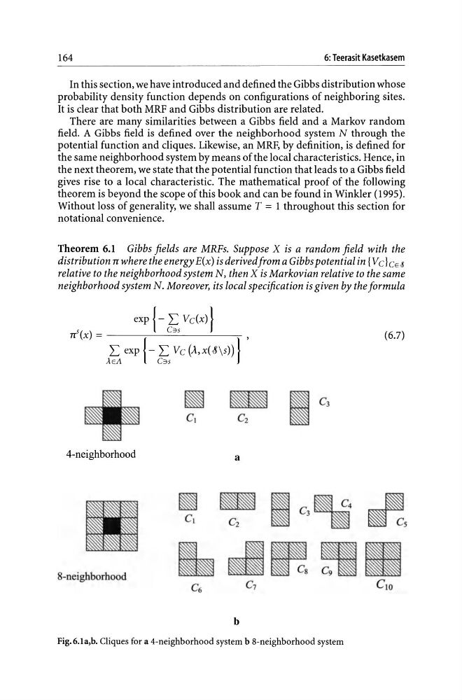
Fig. 6. 1 a,b. Cliques for a 4-neighborhood system b 8-neighborhood system
6: Teerasit Kasetkasem
In this section, we have introduced and defined the Gibbs distribution whose
probability density function depends on configurations of neighboring sites.
It is clear that both MRF and Gibbs distribution are related.
There are many similarities between a Gibbs field and a Markov random
field. A Gibbs field is defined over the neighborhood system N through the
potential function and cliques. Likewise, an MRF, by definition, is defined for
the same neighborhood system by means of the local characteristics. Hence, in
the next theorem, we state that the potential function that leads to a Gibbs field
gives rise to a local characteristic. The mathematical proof of the following
theorem is beyond the scope of this book and can be found in Winkler (1995).
Without loss of generality, we shall assume T = 1 throughout this section for
notational convenience.
Theorem 6.1 Gibbs fields are MRFs. Suppose X is a random field with the
distribution Trwhere the energy E(x) is derived from a Gibbs potential in {V C }CES
relative to the neighborhood system N, then X is Markovian relative to the same
neighborhood system N. Moreover, its local specification is given by the formula
exp {- L Vc(X)}
Jt(x) =
C35
L exp {- L Vc (A,X(J \ S))} ,
AEA
C3S
(6.7)
4-neighborhood
a
~ I C3 ~' ~5
8-neighborhood
~dl'~
b
Fig. 6. 1 a,b. Cliques for a 4-neighborhood system b 8-neighborhood system