

66
3 Numerical Implementation of the Wave Energy Balance Equation
To integrate numerically the right-hand side of the wave energy balance
equation, a number of first and second order explicit and implicit numerical
schemes (Ocean Wave Modeling, 1985; Ryvkin, 1990) are used, including
different Runge--Kutta schemes. It should be noted that the use of highorder numerical schemes requires a lot of CPU time, so they are ineffective
for wind wave operational models.
The problem is that different wind wave spectrum bands are developed
with a different rate, depending on the wind speed and wave frequency. As
a result, the processes of high-frequency spectrum band formation happen
quite rapidly. Their numerical calculation requires a sufficiently small time
step that leads to increasing the number of steps and computing time.
This problem is solved differently in numerical models. In most cases some
definite limits are used to restrict the increase of the spectrum value in the
high-frequency bands (Ocean Wave Modeling, 1985).
In the numerical implementation of the WAM model (The WAM model,
1988; Komen et al., 1994) the spectrum is divided into two ranges: a prognostic one, covering both the maximum area and the low-frequency band,
and a diagnostic one, covering the spectral high-frequency tail. The two conditions are imposed on the spectral value in the second range. The first one
consists in prescribing the dependence of the spectral energy density, such as
S(w) "'u,·- 5 , starting with some definite frequency. In addition, the evolution
rate of the wave energy spectral density (or the source function value) should
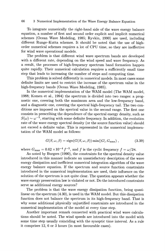
not exceed a definite value. This is represented in the numerical implementation of the WAM model as follows:
G(S, w, (3) = sign(G(S, w, (3)) min(IGI, Gmax) ,
(3.39)
where Gmax = 0.62 x 10- 4 f- 5 , and f is the cyclic frequency f = wj2n.
As noted by Burgers (1990), the constraints for the spectral density value
introduced in this manner indicate an unsatisfactory description of the wave
energy dissipation and inefficient numerical integration algorithm of the wave
energy balance equation. If the spectrum and source function constraints
introduced in the numerical implementation are used, their influence on the
solution of the spectrum is not quite clear. The question appears whether the
wave energy preservation law is violated or not. Do the introduced constraints
serve as additional energy sources?
The problem is that the wave energy dissipation function, being quasilinear on the spectrum (4.30), is used in the WAM model. But this dissipation
function does not balance the spectrum in its high-frequency band. That is
why some additional physically unjustified constraints are introduced in the
numerical implementation of the model at every time step.
Another important remark connected with practical wind wave calculations should be noted. The wind speeds are introduced into the model with
some time step usually coinciding with the synoptic time interval. As a rule
it comprises 12, 6 or 3 hours (in most favourable cases).
3 Numerical Implementation of the Wave Energy Balance Equation
To integrate numerically the right-hand side of the wave energy balance
equation, a number of first and second order explicit and implicit numerical
schemes (Ocean Wave Modeling, 1985; Ryvkin, 1990) are used, including
different Runge--Kutta schemes. It should be noted that the use of highorder numerical schemes requires a lot of CPU time, so they are ineffective
for wind wave operational models.
The problem is that different wind wave spectrum bands are developed
with a different rate, depending on the wind speed and wave frequency. As
a result, the processes of high-frequency spectrum band formation happen
quite rapidly. Their numerical calculation requires a sufficiently small time
step that leads to increasing the number of steps and computing time.
This problem is solved differently in numerical models. In most cases some
definite limits are used to restrict the increase of the spectrum value in the
high-frequency bands (Ocean Wave Modeling, 1985).
In the numerical implementation of the WAM model (The WAM model,
1988; Komen et al., 1994) the spectrum is divided into two ranges: a prognostic one, covering both the maximum area and the low-frequency band,
and a diagnostic one, covering the spectral high-frequency tail. The two conditions are imposed on the spectral value in the second range. The first one
consists in prescribing the dependence of the spectral energy density, such as
S(w) "'u,·- 5 , starting with some definite frequency. In addition, the evolution
rate of the wave energy spectral density (or the source function value) should
not exceed a definite value. This is represented in the numerical implementation of the WAM model as follows:
G(S, w, (3) = sign(G(S, w, (3)) min(IGI, Gmax) ,
(3.39)
where Gmax = 0.62 x 10- 4 f- 5 , and f is the cyclic frequency f = wj2n.
As noted by Burgers (1990), the constraints for the spectral density value
introduced in this manner indicate an unsatisfactory description of the wave
energy dissipation and inefficient numerical integration algorithm of the wave
energy balance equation. If the spectrum and source function constraints
introduced in the numerical implementation are used, their influence on the
solution of the spectrum is not quite clear. The question appears whether the
wave energy preservation law is violated or not. Do the introduced constraints
serve as additional energy sources?
The problem is that the wave energy dissipation function, being quasilinear on the spectrum (4.30), is used in the WAM model. But this dissipation
function does not balance the spectrum in its high-frequency band. That is
why some additional physically unjustified constraints are introduced in the
numerical implementation of the model at every time step.
Another important remark connected with practical wind wave calculations should be noted. The wind speeds are introduced into the model with
some time step usually coinciding with the synoptic time interval. As a rule
it comprises 12, 6 or 3 hours (in most favourable cases).