

3.7 Numerical Integration of the Source Function
65
r.(t)
1.2.-a~~--------------,
o~~--~~--~~
Mr-~~-------------,
55
10
20 30 +0
50
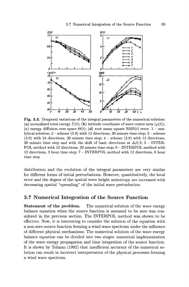
Fig. 3.3. Temporal variations of the integral parameters of the numerical solution:
(a) normalized total energy E(t); (b) latitude coordinate of wave centre area (rp(t));
(c) energy diffusion over space B(t); (d) root mean square RMS(t) error. 1- analytical solution; 2- scheme (3.9) with 12 directions, 20 minute time step; 3- scheme
(3.9) with 24 directions, 20 minute time step; 4 - scheme (3.9) with 12 directions,
20 minute time step and with the shift of basic directions at !:::..(3 /2; 5 - INTERPOL method with 12 directions, 20 minute time step; 6 - INTERPOL method with
12 directions, 3 hour time step; 7- INTERPOL method with 12 directions, 6 hour
time step
distribution and the evolution of the integral parameters are very similar
for different forms of initial perturbations. However, quantitatively, the local
error and the degree of the spatial wave height anisotropy are increased with
decreasing spatial "spreading" of the initial wave perturbation.
3.7 Numerical Integration of the Source Function
Statement of the problem. The numerical solution of the wave energy
balance equation when the source function is assumed to be zero was considered in the previous section. The INTERPOL method was shown to be
effective. Now, it is interesting to consider the solution of the equation with
a non-zero source function forming a wind wave spectrum under the influence
of different physical mechanisms. The numerical solution of the wave energy
balance equation can be divided into two stages: numerical implementation
of the wave energy propagation and time integration of the source function.
It is shown by Tolman (1992) that insufficient accuracy of the numerical solution can result in incorrect interpretation of the physical processes forming
a wind wave spectrum.
65
r.(t)
1.2.-a~~--------------,
o~~--~~--~~
Mr-~~-------------,
55
10
20 30 +0
50
Fig. 3.3. Temporal variations of the integral parameters of the numerical solution:
(a) normalized total energy E(t); (b) latitude coordinate of wave centre area (rp(t));
(c) energy diffusion over space B(t); (d) root mean square RMS(t) error. 1- analytical solution; 2- scheme (3.9) with 12 directions, 20 minute time step; 3- scheme
(3.9) with 24 directions, 20 minute time step; 4 - scheme (3.9) with 12 directions,
20 minute time step and with the shift of basic directions at !:::..(3 /2; 5 - INTERPOL method with 12 directions, 20 minute time step; 6 - INTERPOL method with
12 directions, 3 hour time step; 7- INTERPOL method with 12 directions, 6 hour
time step
distribution and the evolution of the integral parameters are very similar
for different forms of initial perturbations. However, quantitatively, the local
error and the degree of the spatial wave height anisotropy are increased with
decreasing spatial "spreading" of the initial wave perturbation.
3.7 Numerical Integration of the Source Function
Statement of the problem. The numerical solution of the wave energy
balance equation when the source function is assumed to be zero was considered in the previous section. The INTERPOL method was shown to be
effective. Now, it is interesting to consider the solution of the equation with
a non-zero source function forming a wind wave spectrum under the influence
of different physical mechanisms. The numerical solution of the wave energy
balance equation can be divided into two stages: numerical implementation
of the wave energy propagation and time integration of the source function.
It is shown by Tolman (1992) that insufficient accuracy of the numerical solution can result in incorrect interpretation of the physical processes forming
a wind wave spectrum.