

7.5 Surface Gravity Wave Interaction with Elastic Ice Floes
341
any reflection. According to Meylan & Squire (1994), these zeros are called
resonance points.
If L j >. » 1, the distance between the resonance points tends to half
a wavelength beneath the ice. In the case of small plate lengths the structure
of the curve is disturbed. This may be attributed to fringe effects on the
penetration of a wave under ice cover. As shown by calculation, these effects
become noticeable at plate lengths less than the value c1>.' (where >.' is the
wavelength beneath the ice, c1 = 0.80-Q.85 is an empirical coefficient). The
absolute value of the reflection coefficient is calculated to reach a maximum
for the following relationship between the wave and plate lengths: L ;:::j c2 >.2
(c2 = 0.55-0.60).
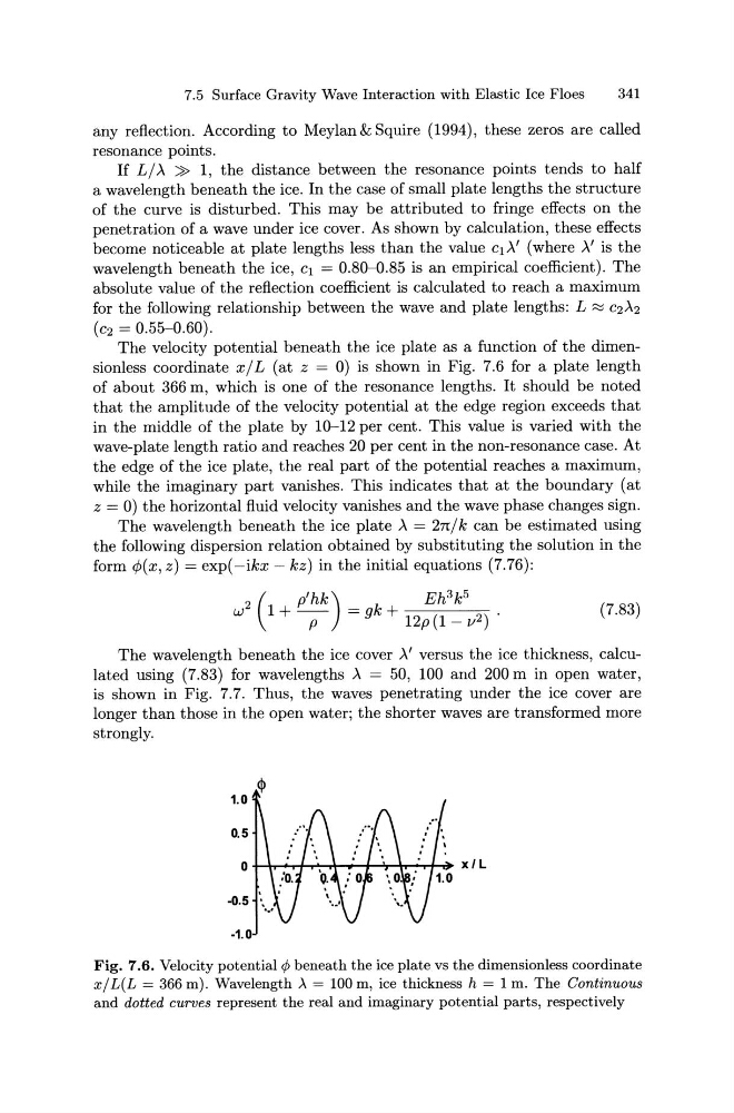
The velocity potential beneath the ice plate as a function of the dimensionless coordinate xj L (at z = 0) is shown in Fig. 7.6 for a plate length
of about 366 m, which is one of the resonance lengths. It should be noted
that the amplitude of the velocity potential at the edge region exceeds that
in the middle of the plate by 10-12 per cent. This value is varied with the
wave-plate length ratio and reaches 20 per cent in the non-resonance case. At
the edge of the ice plate, the real part of the potential reaches a maximum,
while the imaginary part vanishes. This indicates that at the boundary (at
z = 0) the horizontal fluid velocity vanishes and the wave phase changes sign.
The wavelength beneath the ice plate >. = 2n/ k can be estimated using
the following dispersion relation obtained by substituting the solution in the
form ¢(x, z) = exp( -ikx- kz) in the initial equations (7. 76):
2 (
p'hk)
Eh 3 k 5
w 1 + p = gk + 12p (1 - v2) .
(7.83)
The wavelength beneath the ice cover >.' versus the ice thickness, calculated using (7.83) for wavelengths >. = 50, 100 and 200m in open water,
is shown in Fig. 7.7. Thus, the waves penetrating under the ice cover are
longer than those in the open water; the shorter waves are transformed more
strongly.
1.0
0.5
0
x/L
-0.5
-1.0
Fig. 7.6. Velocity potential rjJ beneath the ice plate vs the dimensionless coordinate
xj L(L = 366m). Wavelength >. = 100m, ice thickness h = 1m. The Continuous
and dotted curves represent the real and imaginary potential parts, respectively
341
any reflection. According to Meylan & Squire (1994), these zeros are called
resonance points.
If L j >. » 1, the distance between the resonance points tends to half
a wavelength beneath the ice. In the case of small plate lengths the structure
of the curve is disturbed. This may be attributed to fringe effects on the
penetration of a wave under ice cover. As shown by calculation, these effects
become noticeable at plate lengths less than the value c1>.' (where >.' is the
wavelength beneath the ice, c1 = 0.80-Q.85 is an empirical coefficient). The
absolute value of the reflection coefficient is calculated to reach a maximum
for the following relationship between the wave and plate lengths: L ;:::j c2 >.2
(c2 = 0.55-0.60).
The velocity potential beneath the ice plate as a function of the dimensionless coordinate xj L (at z = 0) is shown in Fig. 7.6 for a plate length
of about 366 m, which is one of the resonance lengths. It should be noted
that the amplitude of the velocity potential at the edge region exceeds that
in the middle of the plate by 10-12 per cent. This value is varied with the
wave-plate length ratio and reaches 20 per cent in the non-resonance case. At
the edge of the ice plate, the real part of the potential reaches a maximum,
while the imaginary part vanishes. This indicates that at the boundary (at
z = 0) the horizontal fluid velocity vanishes and the wave phase changes sign.
The wavelength beneath the ice plate >. = 2n/ k can be estimated using
the following dispersion relation obtained by substituting the solution in the
form ¢(x, z) = exp( -ikx- kz) in the initial equations (7. 76):
2 (
p'hk)
Eh 3 k 5
w 1 + p = gk + 12p (1 - v2) .
(7.83)
The wavelength beneath the ice cover >.' versus the ice thickness, calculated using (7.83) for wavelengths >. = 50, 100 and 200m in open water,
is shown in Fig. 7.7. Thus, the waves penetrating under the ice cover are
longer than those in the open water; the shorter waves are transformed more
strongly.
1.0
0.5
0
x/L
-0.5
-1.0
Fig. 7.6. Velocity potential rjJ beneath the ice plate vs the dimensionless coordinate
xj L(L = 366m). Wavelength >. = 100m, ice thickness h = 1m. The Continuous
and dotted curves represent the real and imaginary potential parts, respectively