

7.3 Kinetic Equation for Non-linear Waves in Sea with Ice Cakes
327
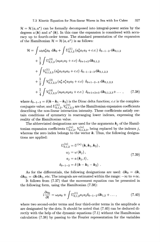
1{ = 1{ (a, a*) can be formally decomposed into integral-power series by the
degrees a (k) and a* (k). In this case the expansion is considered with accuracy up to fourth-order terms. The standard presentation of the expansion
of the Hamiltonian 1i = 1i (a, a*) is as follows:
1{ = J Woa~ao dko + J u6~,2 (a~a1a2 + c.c.) Oo-1-2 dko,1,2
1 J (3)
+ 3 U0,1,2 (aoa1a2 + c.c) Oo+H2dk0,1,2
+ J V0\i~2,3 (a~a1a2a3 + c.c) Oo-l-2-3dko,1,2,3
1 J v;(2) ( * * ) s: dk
+ -
o 1 2 3 ao a1 a2a3 + c.c uo+l-2-3 0,1,2,3
2
' ' '
(7.38)
where 80_ 1_2 = o(k- k 1 - k 2 ) is the Dirac delta function; c.c is the complexconjugate value; and u6n{ 2 , V 0 (~) 2 3 are the Hamiltonian expansion coefficients
describing the non-line~r' inte;~ction intensity. These coefficients satisfy certain conditions of symmetry in rearranging lower indexes, expressing the
reality of the Hamiltonian value.
The abbreviated designations are used for the arguments kj of the Hamiltonian expansion coefficients u6~l 2 , V 0 C~l 2 3 , being replaced by the indexes j,
whereas the zero index belongs t~ the ~~~tor k. Thus, the following designations are applied:
u6~{,2 = u(n) (k, k1, kz)'
wj=w(k 1 ),
aj =a(kj,t),
Oo-1-2 = o (k- k1 - kz)
(7.39)
As for the differentials, the following designations are used: dk0 = dk,
dk01 = dk dk1, etc. The integrals are estimated within the range: -oo to +oo.
It follows from (7.37) that the movement equation can be presented in
the following form, using the Hamiltonian (7.38):
.&ao _
J (1)
1 &t - woao + U0,1,2a1 a28o-1-2 dk1,2 + ... ,
(7.40)
where two second-order terms and four third-order terms in the amplitude a
are designated by the dots. It should be noted that (7.40) can be deduced directly with the help of the dynamic equations (7.1) without the Hamiltonian
calculation (7.38) by passing to the Fourier representation for the variables
327
1{ = 1{ (a, a*) can be formally decomposed into integral-power series by the
degrees a (k) and a* (k). In this case the expansion is considered with accuracy up to fourth-order terms. The standard presentation of the expansion
of the Hamiltonian 1i = 1i (a, a*) is as follows:
1{ = J Woa~ao dko + J u6~,2 (a~a1a2 + c.c.) Oo-1-2 dko,1,2
1 J (3)
+ 3 U0,1,2 (aoa1a2 + c.c) Oo+H2dk0,1,2
+ J V0\i~2,3 (a~a1a2a3 + c.c) Oo-l-2-3dko,1,2,3
1 J v;(2) ( * * ) s: dk
+ -
o 1 2 3 ao a1 a2a3 + c.c uo+l-2-3 0,1,2,3
2
' ' '
(7.38)
where 80_ 1_2 = o(k- k 1 - k 2 ) is the Dirac delta function; c.c is the complexconjugate value; and u6n{ 2 , V 0 (~) 2 3 are the Hamiltonian expansion coefficients
describing the non-line~r' inte;~ction intensity. These coefficients satisfy certain conditions of symmetry in rearranging lower indexes, expressing the
reality of the Hamiltonian value.
The abbreviated designations are used for the arguments kj of the Hamiltonian expansion coefficients u6~l 2 , V 0 C~l 2 3 , being replaced by the indexes j,
whereas the zero index belongs t~ the ~~~tor k. Thus, the following designations are applied:
u6~{,2 = u(n) (k, k1, kz)'
wj=w(k 1 ),
aj =a(kj,t),
Oo-1-2 = o (k- k1 - kz)
(7.39)
As for the differentials, the following designations are used: dk0 = dk,
dk01 = dk dk1, etc. The integrals are estimated within the range: -oo to +oo.
It follows from (7.37) that the movement equation can be presented in
the following form, using the Hamiltonian (7.38):
.&ao _
J (1)
1 &t - woao + U0,1,2a1 a28o-1-2 dk1,2 + ... ,
(7.40)
where two second-order terms and four third-order terms in the amplitude a
are designated by the dots. It should be noted that (7.40) can be deduced directly with the help of the dynamic equations (7.1) without the Hamiltonian
calculation (7.38) by passing to the Fourier representation for the variables