328
7 Wave Transformation in Ice-Covered Water
TJ (k) and x (k). Evidence of canonical conjugation for the couple of variables TJ (:v, t), x (:v, t) may be considered to obtain equations coinciding with
each other with an accuracy up to complex conjugation after passing to the
normal variables a(k), a*(k) and proper symmetrization of the interaction
coefficients. The same expansion coefficients occur in the final equation as in
(7.40).
Expansion coefficients of the Hamiltonian. The technique described
by Krasitskii & Kalmykov (1993) for water without ice is used below.
The general solution of the Laplace equation, satisfying the bottom
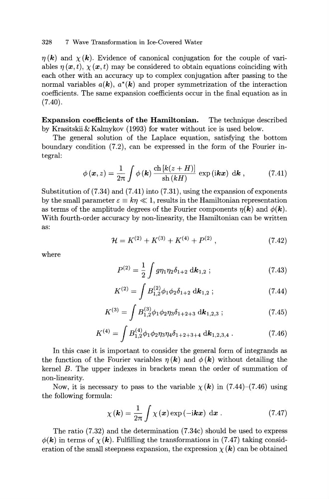
boundary condition (7.2), can be expressed in the form of the Fourier integral:
1 J ch[k(z+H)] .
(:v,z) = 2rr (k) sh(kH)
exp(Ik:v) dk'
(7.41)
Substitution of (7.34) and (7.41) into (7.31), using the expansion of exponents
by the small parameter c: = kry « 1, results in the Hamiltonian representation
as terms of the amplitude degrees of the Fourier components ry(k) and (k).
With fourth-order accuracy by non-linearity, the Hamiltonian can be written
as:
where
1l = K{2) + K{3) + K{4) + p{2) ,
p( 2 ) = ~ J g'T}l'fJ2bH2 dk1,2 ;
K< 2 l = J B~~~1261+2 dk1,2 ;
K( 3 ) = J B~~~12'T}36H2+3 dk1,2,3 ;
K( 4 ) = J B~~~12'TJ3'TJ4bH2+3+4 dk1,2,3,4 ·
(7.42)
(7.43)
(7.44)
(7.45)
(7.46)
In this case it is important to consider the general form of integrands as
the function of the Fourier variables TJ ( k) and ( k) without detailing the
kernel B. The upper indexes in brackets mean the order of summation of
non-linearity.
Now, it is necessary to pass to the variable x (k) in (7.44)-(7.46) using
the following formula:
x(k) = _!__jx(:v)exp(-ik:v) d:v.
2rr
(7.47)
The ratio (7.32) and the determination (7.34c) should be used to express
(k) in terms of x (k). Fulfilling the transformations in (7.47) taking consideration of the small steepness expansion, the expression X (k) can be obtained