

6.4 Wave Energy Dissipation in Shallow Water
287
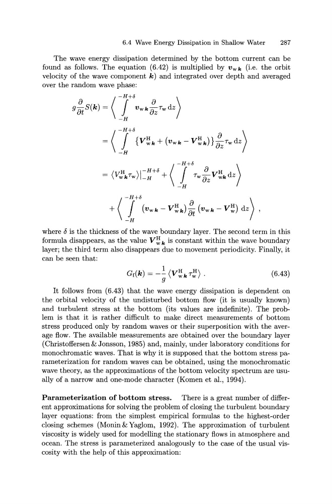
The wave energy dissipation determined by the bottom current can be
found as follows. The equation (6.42) is multiplied by Vwk (i.e. the orbit
velocity of the wave component k) and integrated over depth and averaged
over the random wave phase:
H
-H +o ( -~H +6 0 H )
= (Vwkrw)j_H +
Tw 0 zVwkdz
-H
+ ( T'(vw.- v~.)! (vw.- V~) dz) '
-H
where 8 is the thickness of the wave boundary layer. The second term in this
formula disappears, as the value V~ k is constant within the wave boundary
layer; the third term also disappears due to movement periodicity. Finally, it
can be seen that:
(6.43)
It follows from (6.43) that the wave energy dissipation is dependent on
the orbital velocity of the undisturbed bottom flow (it is usually known)
and turbulent stress at the bottom (its values are indefinite). The problem is that it is rather difficult to make direct measurements of bottom
stress produced only by random waves or their superposition with the average flow. The available measurements are obtained over the boundary layer
(Christoffersen & Jonsson, 1985) and, mainly, under laboratory conditions for
monochromatic waves. That is why it is supposed that the bottom stress parameterization for random waves can be obtained, using the monochromatic
wave theory, as the approximations of the bottom velocity spectrum are usually of a narrow and one-mode character (Kamen et al., 1994).
Parameterization of bottom stress. There is a great number of different approximations for solving the problem of closing the turbulent boundary
layer equations: from the simplest empirical formulas to the highest-order
closing schemes (Monin&Yaglom, 1992). The approximation of turbulent
viscosity is widely used for modelling the stationary flows in atmosphere and
ocean. The stress is parameterized analogously to the case of the usual viscosity with the help of this approximation:
287
The wave energy dissipation determined by the bottom current can be
found as follows. The equation (6.42) is multiplied by Vwk (i.e. the orbit
velocity of the wave component k) and integrated over depth and averaged
over the random wave phase:
H
-H +o ( -~H +6 0 H )
= (Vwkrw)j_H +
Tw 0 zVwkdz
-H
+ ( T'(vw.- v~.)! (vw.- V~) dz) '
-H
where 8 is the thickness of the wave boundary layer. The second term in this
formula disappears, as the value V~ k is constant within the wave boundary
layer; the third term also disappears due to movement periodicity. Finally, it
can be seen that:
(6.43)
It follows from (6.43) that the wave energy dissipation is dependent on
the orbital velocity of the undisturbed bottom flow (it is usually known)
and turbulent stress at the bottom (its values are indefinite). The problem is that it is rather difficult to make direct measurements of bottom
stress produced only by random waves or their superposition with the average flow. The available measurements are obtained over the boundary layer
(Christoffersen & Jonsson, 1985) and, mainly, under laboratory conditions for
monochromatic waves. That is why it is supposed that the bottom stress parameterization for random waves can be obtained, using the monochromatic
wave theory, as the approximations of the bottom velocity spectrum are usually of a narrow and one-mode character (Kamen et al., 1994).
Parameterization of bottom stress. There is a great number of different approximations for solving the problem of closing the turbulent boundary
layer equations: from the simplest empirical formulas to the highest-order
closing schemes (Monin&Yaglom, 1992). The approximation of turbulent
viscosity is widely used for modelling the stationary flows in atmosphere and
ocean. The stress is parameterized analogously to the case of the usual viscosity with the help of this approximation: