

56
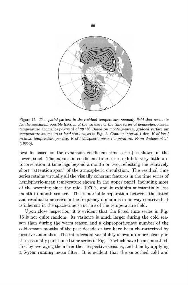
Figure 15: The spatial pattern in the residual temperature anomaly field that accounts
for the maximum possible fraction of the variance of the time series of hemispheric-mean
temperature anomalies poleward of 20 0 N. Based on monthly-mean, gridded surface air
temperature anomalies at land stations, as in Fig. 2. Contour interval 1 deg. K of local
residual temperature per deg. K of hemispheric mean temperature. From Wallace et al.
(1995b) .
best fit based on the expansion coefficient time series) is shown in the
lower panel. The expansion coefficient time series exhibits very little autocorrelation at time lags beyond a month or two, reflecting the relatively
short "attention span" of the atmospheric circulation. The residual time
series retains virtually all the visually coherent features in the time series of
hemispheric-mean temperature shown in the upper panel, including most
of the warming since the mid- 1970's, and it exhibits substantially less
month-to-month scatter. The remarkable separation between the fitted
and residual time series in the frequency domain is in no way contrived: it
is inherent in the space-time structure of the temperature field.
Upon close inspection, it is evident that the fitted time series in Fig.
16 is not quite random. Its variance is much larger during the cold season than during the warm season and a disproportionate number of the
cold-season months of the past decade or two have been characterized by
positive anomalies. The interdecadal variability shows up more clearly in
the seasonally partitioned time series in Fig. 17 which have been smoothed,
first by averaging them over their respective seasons, and then by applying
a 5-year running mean filter. It is evident that the smoothed cold and
Figure 15: The spatial pattern in the residual temperature anomaly field that accounts
for the maximum possible fraction of the variance of the time series of hemispheric-mean
temperature anomalies poleward of 20 0 N. Based on monthly-mean, gridded surface air
temperature anomalies at land stations, as in Fig. 2. Contour interval 1 deg. K of local
residual temperature per deg. K of hemispheric mean temperature. From Wallace et al.
(1995b) .
best fit based on the expansion coefficient time series) is shown in the
lower panel. The expansion coefficient time series exhibits very little autocorrelation at time lags beyond a month or two, reflecting the relatively
short "attention span" of the atmospheric circulation. The residual time
series retains virtually all the visually coherent features in the time series of
hemispheric-mean temperature shown in the upper panel, including most
of the warming since the mid- 1970's, and it exhibits substantially less
month-to-month scatter. The remarkable separation between the fitted
and residual time series in the frequency domain is in no way contrived: it
is inherent in the space-time structure of the temperature field.
Upon close inspection, it is evident that the fitted time series in Fig.
16 is not quite random. Its variance is much larger during the cold season than during the warm season and a disproportionate number of the
cold-season months of the past decade or two have been characterized by
positive anomalies. The interdecadal variability shows up more clearly in
the seasonally partitioned time series in Fig. 17 which have been smoothed,
first by averaging them over their respective seasons, and then by applying
a 5-year running mean filter. It is evident that the smoothed cold and