

454
0.4 ,-----~------_,------~------._------~----_.
C\I
I
,...
0.3
0.2
0.1
u.
0.0
o -0.1
l.U -0.2
-0.3
-0.4
0.3
,.
0.2
('I)
0.1
u.
0.0
o -0.1
l.U -0.2
-0.3
- - EOF1
- - EOF2
-0.4 L-L~~-----'-----'--~~-'--~~--'-----"~---,--~-----'-----,--~~---L-~~---'------.!
o
10
20
30
Rankk
40
50
60
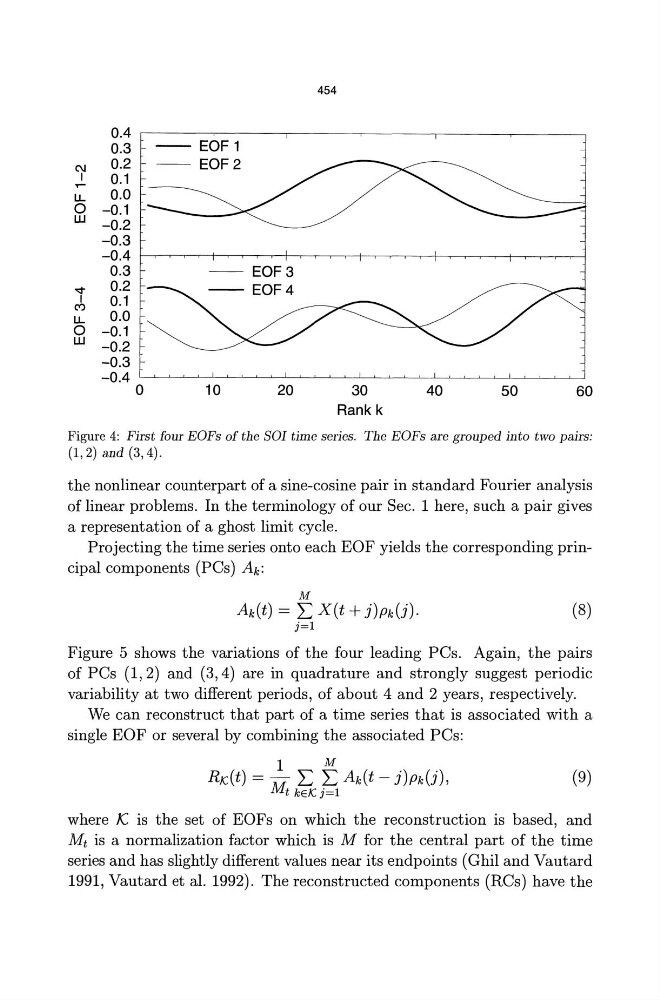
Figure 4: First four EOFs of the SOl time series. The EOFs are grouped into two pairs:
(1,2) and (3,4).
the nonlinear counterpart of a sine-cosine pair in standard Fourier analysis
of linear problems. In the terminology of our Sec. 1 here, such a pair gives
a representation of a ghost limit cycle.
Projecting the time series onto each EOF yields the corresponding principal components (PCs) Ak :
M
Ak(t) = L X(t + j)pkU),
j=l
(8)
Figure 5 shows the variations of the four leading PCs. Again, the pairs
of PCs (1,2) and (3,4) are in quadrature and strongly suggest periodic
variability at two different periods, of about 4 and 2 years, respectively.
We can reconstruct that part of a time series that is associated with a
single EOF or several by combining the associated PCs:
RK.(t) = M1 L I: Ak(t - j)PkU),
t kEIC j=l
(9)
where J( is the set of EOFs on which the reconstruction is based, and
M t is a normalization factor which is M for the central part of the time
series and has slightly different values near its endpoints (Ghil and Vautard
1991, Vautard et al. 1992). The reconstructed components (RCs) have the
0.4 ,-----~------_,------~------._------~----_.
C\I
I
,...
0.3
0.2
0.1
u.
0.0
o -0.1
l.U -0.2
-0.3
-0.4
0.3
,.
0.2
('I)
0.1
u.
0.0
o -0.1
l.U -0.2
-0.3
- - EOF1
- - EOF2
-0.4 L-L~~-----'-----'--~~-'--~~--'-----"~---,--~-----'-----,--~~---L-~~---'------.!
o
10
20
30
Rankk
40
50
60
Figure 4: First four EOFs of the SOl time series. The EOFs are grouped into two pairs:
(1,2) and (3,4).
the nonlinear counterpart of a sine-cosine pair in standard Fourier analysis
of linear problems. In the terminology of our Sec. 1 here, such a pair gives
a representation of a ghost limit cycle.
Projecting the time series onto each EOF yields the corresponding principal components (PCs) Ak :
M
Ak(t) = L X(t + j)pkU),
j=l
(8)
Figure 5 shows the variations of the four leading PCs. Again, the pairs
of PCs (1,2) and (3,4) are in quadrature and strongly suggest periodic
variability at two different periods, of about 4 and 2 years, respectively.
We can reconstruct that part of a time series that is associated with a
single EOF or several by combining the associated PCs:
RK.(t) = M1 L I: Ak(t - j)PkU),
t kEIC j=l
(9)
where J( is the set of EOFs on which the reconstruction is based, and
M t is a normalization factor which is M for the central part of the time
series and has slightly different values near its endpoints (Ghil and Vautard
1991, Vautard et al. 1992). The reconstructed components (RCs) have the