

453
its columns and the diagonal matrix Ax composed of the eigenvalues Ak,
in deceasing order:
ESr.Cx Ex = Ax,
(7)
where E~ is the transpose of Ex. Each eigenvalue Ak gives the degree of
extension (and hence the variance) of the time series in the direction given
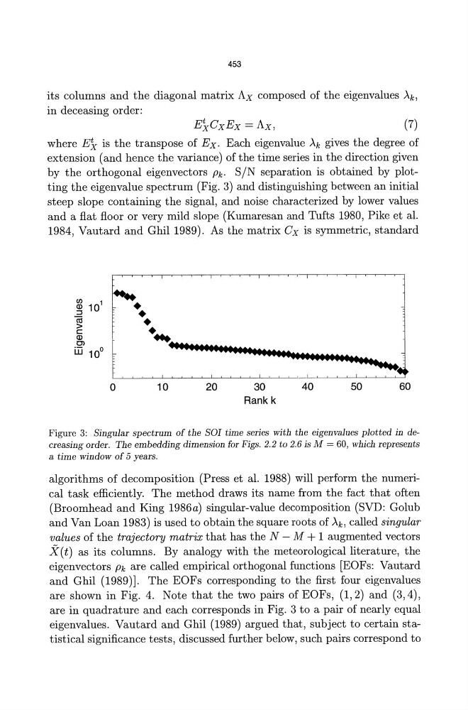
by the orthogonal eigenvectors Pk. SIN separation is obtained by plotting the eigenvalue spectrum (Fig. 3) and distinguishing between an initial
steep slope containing the signal, and noise characterized by lower values
and a flat floor or very mild slope (Kumaresan and Tufts 1980, Pike et al.
1984, Vautard and Ghil 1989). As the matrix Cx is symmetric, standard
~ .
• • .... ..... ~.~.~ .... ~.".~ .... ~." ...... ".~ ....•. ".~.~~~~~~~~~ .
••••••••••••••••••
~ ..... ~
o
10
20
30
40
50
60
Rank k
Figure 3: Singular spectrum of the SOl time series with the eigenvalues plotted in decreasing order. The embedding dimension for Figs. 2.2 to 2.6 is M = 60, which represents
a time window of 5 years.
algorithms of decomposition (Press et al. 1988) will perform the numerical task efficiently. The method draws its name from the fact that often
(Broomhead and King 1986a) singular-value decomposition (SVD: Golub
and Van Loan 1983) is used to obtain the square roots of Ak, called singular
values of the trajectory matrix that has the N - M + 1 augmented vectors
X(t) as its columns. By analogy with the meteorological literature, the
eigenvectors Pk are called empirical orthogonal functions [EOFs: Vautard
and Ghil (1989)]. The EOFs corresponding to the first four eigenvalues
are shown in Fig. 4. Note that the two pairs of EOFs, (1,2) and (3,4),
are in quadrature and each corresponds in Fig. 3 to a pair of nearly equal
eigenvalues. Vautard and Ghil (1989) argued that, subject to certain statistical significance tests, discussed further below, such pairs correspond to
its columns and the diagonal matrix Ax composed of the eigenvalues Ak,
in deceasing order:
ESr.Cx Ex = Ax,
(7)
where E~ is the transpose of Ex. Each eigenvalue Ak gives the degree of
extension (and hence the variance) of the time series in the direction given
by the orthogonal eigenvectors Pk. SIN separation is obtained by plotting the eigenvalue spectrum (Fig. 3) and distinguishing between an initial
steep slope containing the signal, and noise characterized by lower values
and a flat floor or very mild slope (Kumaresan and Tufts 1980, Pike et al.
1984, Vautard and Ghil 1989). As the matrix Cx is symmetric, standard
~ .
• • .... ..... ~.~.~ .... ~.".~ .... ~." ...... ".~ ....•. ".~.~~~~~~~~~ .
••••••••••••••••••
~ ..... ~
o
10
20
30
40
50
60
Rank k
Figure 3: Singular spectrum of the SOl time series with the eigenvalues plotted in decreasing order. The embedding dimension for Figs. 2.2 to 2.6 is M = 60, which represents
a time window of 5 years.
algorithms of decomposition (Press et al. 1988) will perform the numerical task efficiently. The method draws its name from the fact that often
(Broomhead and King 1986a) singular-value decomposition (SVD: Golub
and Van Loan 1983) is used to obtain the square roots of Ak, called singular
values of the trajectory matrix that has the N - M + 1 augmented vectors
X(t) as its columns. By analogy with the meteorological literature, the
eigenvectors Pk are called empirical orthogonal functions [EOFs: Vautard
and Ghil (1989)]. The EOFs corresponding to the first four eigenvalues
are shown in Fig. 4. Note that the two pairs of EOFs, (1,2) and (3,4),
are in quadrature and each corresponds in Fig. 3 to a pair of nearly equal
eigenvalues. Vautard and Ghil (1989) argued that, subject to certain statistical significance tests, discussed further below, such pairs correspond to