

452
as well as interannual (Rasmusson et al. 1990, Keppenne and Ghil 1992)
and intraseasonal (Ghil and Mo 1991a,b) oscillations. SSA algorithms and
their properties have been investigated further by Penland et al. (1991),
Allen (1992) and Vautard et al. (1992). The software of Dettinger et al.
(1995a) is built, mainly but not exclusively, around this technique.
2.2 Decomposition and reconstruction
In this section, we illustrate the fundamental SSA formulae with a classical
example of a climatic time series, the Southern Oscillation Index (SOl).
SOl is a climatic index connected with the recurring El Nino conditions
in the tropical Pacific; it is essentially the monthly mean difference in sealevel pressure between Darwin, Australia and Tahiti. In the data set we
use here, the annual cycle was removed and the time series was normalized
by its variance. The time interval considered goes from January 1942 to
December 1990, during which no observations are missing at either station.
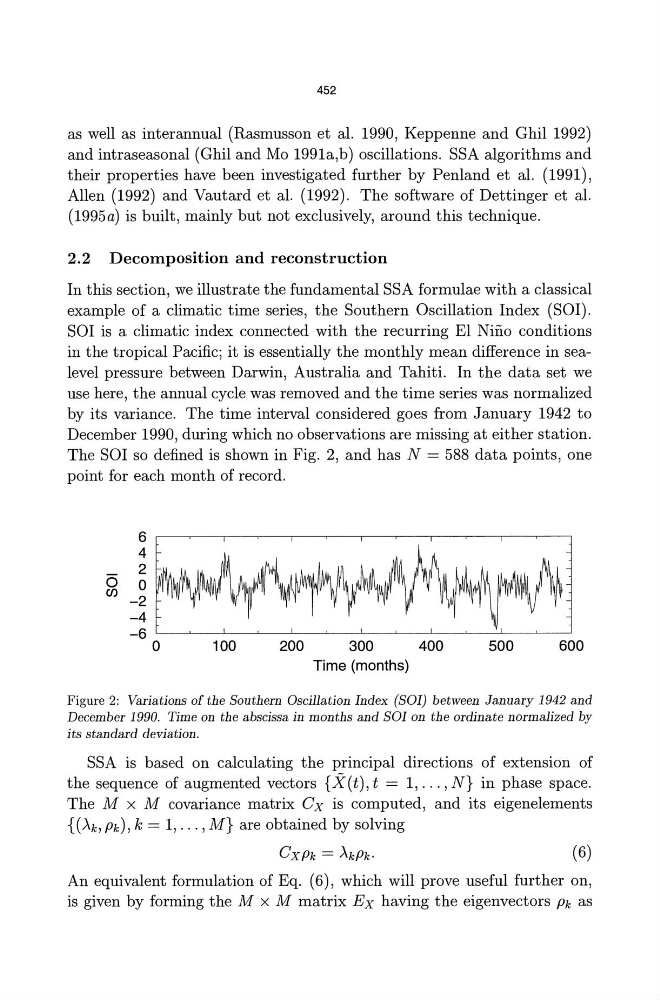
The SOl so defined is shown in Fig. 2, and has N = 588 data points, one
point for each month of record.
6
4
2
6 0
en -2
-4
-6
o
100
200
300
Time (months)
400
500
600
Figure 2: Variations of the Southern Oscillation Index (SOl) between January 1942 and
December 1990. Time on the abscissa in months and SOlon the ordinate normalized by
its standard deviation.
SSA is based on calculating the principal directions of extension of
the sequence of augmented vectors {X(t), t = 1, ... , N} in phase space.
The M X M covariance matrix ex is computed, and its eigenelements
{(Ak' Pk), k = 1, ... , M} are obtained by solving
CXPk = AkPk.
(6)
An equivalent formulation of Eq. (6), which will prove useful further on,
is given by forming the M x M matrix Ex having the eigenvectors Pk as
as well as interannual (Rasmusson et al. 1990, Keppenne and Ghil 1992)
and intraseasonal (Ghil and Mo 1991a,b) oscillations. SSA algorithms and
their properties have been investigated further by Penland et al. (1991),
Allen (1992) and Vautard et al. (1992). The software of Dettinger et al.
(1995a) is built, mainly but not exclusively, around this technique.
2.2 Decomposition and reconstruction
In this section, we illustrate the fundamental SSA formulae with a classical
example of a climatic time series, the Southern Oscillation Index (SOl).
SOl is a climatic index connected with the recurring El Nino conditions
in the tropical Pacific; it is essentially the monthly mean difference in sealevel pressure between Darwin, Australia and Tahiti. In the data set we
use here, the annual cycle was removed and the time series was normalized
by its variance. The time interval considered goes from January 1942 to
December 1990, during which no observations are missing at either station.
The SOl so defined is shown in Fig. 2, and has N = 588 data points, one
point for each month of record.
6
4
2
6 0
en -2
-4
-6
o
100
200
300
Time (months)
400
500
600
Figure 2: Variations of the Southern Oscillation Index (SOl) between January 1942 and
December 1990. Time on the abscissa in months and SOlon the ordinate normalized by
its standard deviation.
SSA is based on calculating the principal directions of extension of
the sequence of augmented vectors {X(t), t = 1, ... , N} in phase space.
The M X M covariance matrix ex is computed, and its eigenelements
{(Ak' Pk), k = 1, ... , M} are obtained by solving
CXPk = AkPk.
(6)
An equivalent formulation of Eq. (6), which will prove useful further on,
is given by forming the M x M matrix Ex having the eigenvectors Pk as