

450
or fixed points, through stable periodic solutions, or limit cycles, and on
through quasi-periodic solutions lying on tori, to strange attractors. The
fixed points and limit cycles are road posts on this highway from the simple
to the complex and, even after having lost their stability to successively
more complex and realistic solutions, leave their imprint on the observed
spatial patterns or time series generated by the system.
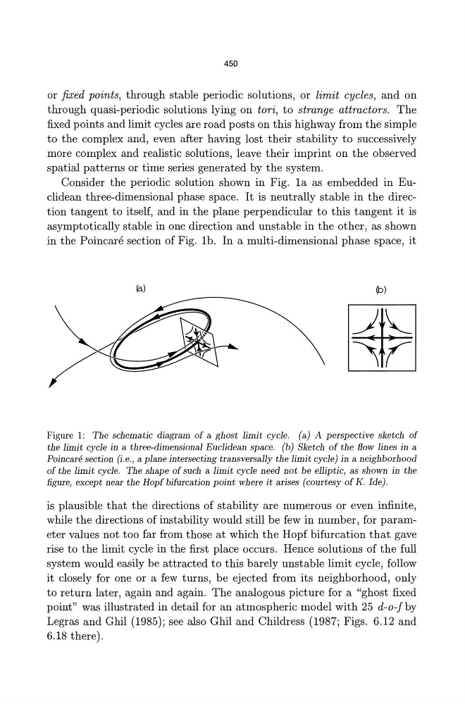
Consider the periodic solution shown in Fig. 1a as embedded in Euclidean three-dimensional phase space. It is neutrally stable in the direction tangent to itself, and in the plane perpendicular to this tangent it is
asymptotically stable in one direction and unstable in the other, as shown
in the Poincare section of Fig. lb. In a multi-dimensional phase space, it
(a)
(b)
Figure 1: The schematic diagram of a ghost limit cycle. (a) A perspective sketch of
the limit cycle in a three-dimensional Euclidean space. (b) Sketch of the flow lines in a
Poincare section (i.e., a plane intersecting transversally the limit cycle) in a neighborhood
of the limit cycle. The shape of such a limit cycle need not be elliptic, as shown in the
figure, except near the Hopf bifurcation point where it arises (courtesy of K. Ide).
is plausible that the directions of stability are numerous or even infinite,
while the directions of instability would still be few in number, for parameter values not too far from those at which the Hopf bifurcation that gave
rise to the limit cycle in the first place occurs. Hence solutions of the full
system would easily be attracted to this barely unstable limit cycle, follow
it closely for one or a few turns, be ejected from its neighborhood, only
to return later, again and again. The analogous picture for a "ghost fixed
point" was illustrated in detail for an atmospheric model with 25 d-o-f by
Legras and Ghil (1985); see also Ghil and Childress (1987; Figs. 6.12 and
6.18 there).
or fixed points, through stable periodic solutions, or limit cycles, and on
through quasi-periodic solutions lying on tori, to strange attractors. The
fixed points and limit cycles are road posts on this highway from the simple
to the complex and, even after having lost their stability to successively
more complex and realistic solutions, leave their imprint on the observed
spatial patterns or time series generated by the system.
Consider the periodic solution shown in Fig. 1a as embedded in Euclidean three-dimensional phase space. It is neutrally stable in the direction tangent to itself, and in the plane perpendicular to this tangent it is
asymptotically stable in one direction and unstable in the other, as shown
in the Poincare section of Fig. lb. In a multi-dimensional phase space, it
(a)
(b)
Figure 1: The schematic diagram of a ghost limit cycle. (a) A perspective sketch of
the limit cycle in a three-dimensional Euclidean space. (b) Sketch of the flow lines in a
Poincare section (i.e., a plane intersecting transversally the limit cycle) in a neighborhood
of the limit cycle. The shape of such a limit cycle need not be elliptic, as shown in the
figure, except near the Hopf bifurcation point where it arises (courtesy of K. Ide).
is plausible that the directions of stability are numerous or even infinite,
while the directions of instability would still be few in number, for parameter values not too far from those at which the Hopf bifurcation that gave
rise to the limit cycle in the first place occurs. Hence solutions of the full
system would easily be attracted to this barely unstable limit cycle, follow
it closely for one or a few turns, be ejected from its neighborhood, only
to return later, again and again. The analogous picture for a "ghost fixed
point" was illustrated in detail for an atmospheric model with 25 d-o-f by
Legras and Ghil (1985); see also Ghil and Childress (1987; Figs. 6.12 and
6.18 there).