

QJ
()
c
1 40
1 20
~ 1 00
'~
()
8 0 80
o
>, 0.60
()
c
QJ
5- 040
QJ
'LL
0.20
125
L
50
2
4.00
9.00'
14.00
Lyopunov Eiponent
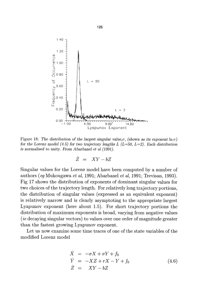
Figure 18: The distribution of the largest singular valuep, (shown as its exponent In (Y)
for the Lorenz model (4.5) for two trajectory lengths L (L=50, L=2). Each distribution
is normalised to unity. From Abarbanel et al (1991).
Z = XY -bZ
Singular values for the Lorenz model have been computed by a number of
authors (eg Mukougawa et al, 1991; Abarbanel et al, 1991; Trevisan, 1993).
Fig 17 shows the distribution of exponents of dominant singular values for
two choices of the trajectory length. For relatively long trajectory portions,
the distribution of singular values (expressed as an equivalent exponent)
is relatively narrow and is clearly asymptoting to the appropriate largest
Lyapunov exponent (here about 1.5). For short trajectory portions the
distribution of maximum exponents is broad, varying from negative values
( ie decaying singular vectors) to values over one order of magnitude greater
than the fastest growing Lyapunov exponent.
Let us now examine some time traces of one of the state variables of the
modified Lorenz model
x
Y
Z
-CJX + CJY + fo
-XZ +rX - Y + fo
XY-bZ
(4.6)
()
c
1 40
1 20
~ 1 00
'~
()
8 0 80
o
>, 0.60
()
c
QJ
5- 040
QJ
'LL
0.20
125
L
50
2
4.00
9.00'
14.00
Lyopunov Eiponent
Figure 18: The distribution of the largest singular valuep, (shown as its exponent In (Y)
for the Lorenz model (4.5) for two trajectory lengths L (L=50, L=2). Each distribution
is normalised to unity. From Abarbanel et al (1991).
Z = XY -bZ
Singular values for the Lorenz model have been computed by a number of
authors (eg Mukougawa et al, 1991; Abarbanel et al, 1991; Trevisan, 1993).
Fig 17 shows the distribution of exponents of dominant singular values for
two choices of the trajectory length. For relatively long trajectory portions,
the distribution of singular values (expressed as an equivalent exponent)
is relatively narrow and is clearly asymptoting to the appropriate largest
Lyapunov exponent (here about 1.5). For short trajectory portions the
distribution of maximum exponents is broad, varying from negative values
( ie decaying singular vectors) to values over one order of magnitude greater
than the fastest growing Lyapunov exponent.
Let us now examine some time traces of one of the state variables of the
modified Lorenz model
x
Y
Z
-CJX + CJY + fo
-XZ +rX - Y + fo
XY-bZ
(4.6)