

538
G. Hanna and A. Sergi
Fig. 14.9 Plot of the
time-dependent coherence,
σ x (t), for the weak
subsystem-field case
(g = 0.1)
-1
-0.5
0
0.5
1
0
20
40
60
80
100
<σ
x >
time
Fig. 14.10 Plot of the
time-dependent coherence,
σ x (t), for the strong
subsystem-field coupling case
(g = 1.5)
-1
-0.5
0
0.5
1
0
20
40
60
80
100
<σ
x >
time
average value of the observable is calculated according to Eq. (14.15), with the use
of the time-dependent basis as opposed to the time-independent one.
The results of the simulations are now presented and discussed. A time step of
τ = 0.1 and 10 5 trajectories were used to obtain all the results. First, the influence
of the driving field on the metamolecule is investigated by varying the subsystemfield coupling from g = 0.1 to g = 1.5 while keeping the system parameters
fixed at β = 12.5, c = 0.01, = 0.8, ω = 0.5 and ω d = 0.05. For this set
of parameter values, the coupling between the quantum dot and resonant mode is
weak, and, therefore, the effect of nonadiabatic transitions (due to this coupling)
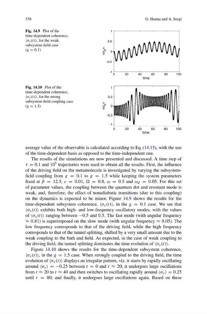
on the dynamics is expected to be minor. Figure 14.9 shows the results for the
time-dependent subsystem coherence, σ x (t), in the g = 0.1 case. We see that
σ x (t) exhibits both high- and low-frequency oscillatory modes, with the values
of σ x (t) ranging between −0.5 and 0.5. The fast mode (with angular frequency
≈ 0.81) is superimposed on the slow mode (with angular frequency ≈ 0.05). The
low frequency corresponds to that of the driving field, while the high frequency
corresponds to that of the tunnel splitting, shifted by a very small amount due to the
weak coupling to the bath and field. As expected, in the case of weak coupling to
the driving field, the tunnel splitting dominates the time evolution of σ x (t).
Figure 14.10 shows the results for the time-dependent subsystem coherence,
σ x (t), in the g = 1.5 case. When strongly coupled to the driving field, the time
evolution of σ x (t) displays an irregular pattern, viz. it starts by rapidly oscillating
around σ x = −0.25 between t = 0 and t ≈ 20; it undergoes large oscillations
from t ≈ 20 to t ≈ 40 and then switches to oscillating rapidly around σ x = 0.25
until t = 80; and finally, it undergoes large oscillations again. Based on these
G. Hanna and A. Sergi
Fig. 14.9 Plot of the
time-dependent coherence,
σ x (t), for the weak
subsystem-field case
(g = 0.1)
-1
-0.5
0
0.5
1
0
20
40
60
80
100
<σ
x >
time
Fig. 14.10 Plot of the
time-dependent coherence,
σ x (t), for the strong
subsystem-field coupling case
(g = 1.5)
-1
-0.5
0
0.5
1
0
20
40
60
80
100
<σ
x >
time
average value of the observable is calculated according to Eq. (14.15), with the use
of the time-dependent basis as opposed to the time-independent one.
The results of the simulations are now presented and discussed. A time step of
τ = 0.1 and 10 5 trajectories were used to obtain all the results. First, the influence
of the driving field on the metamolecule is investigated by varying the subsystemfield coupling from g = 0.1 to g = 1.5 while keeping the system parameters
fixed at β = 12.5, c = 0.01, = 0.8, ω = 0.5 and ω d = 0.05. For this set
of parameter values, the coupling between the quantum dot and resonant mode is
weak, and, therefore, the effect of nonadiabatic transitions (due to this coupling)
on the dynamics is expected to be minor. Figure 14.9 shows the results for the
time-dependent subsystem coherence, σ x (t), in the g = 0.1 case. We see that
σ x (t) exhibits both high- and low-frequency oscillatory modes, with the values
of σ x (t) ranging between −0.5 and 0.5. The fast mode (with angular frequency
≈ 0.81) is superimposed on the slow mode (with angular frequency ≈ 0.05). The
low frequency corresponds to that of the driving field, while the high frequency
corresponds to that of the tunnel splitting, shifted by a very small amount due to the
weak coupling to the bath and field. As expected, in the case of weak coupling to
the driving field, the tunnel splitting dominates the time evolution of σ x (t).
Figure 14.10 shows the results for the time-dependent subsystem coherence,
σ x (t), in the g = 1.5 case. When strongly coupled to the driving field, the time
evolution of σ x (t) displays an irregular pattern, viz. it starts by rapidly oscillating
around σ x = −0.25 between t = 0 and t ≈ 20; it undergoes large oscillations
from t ≈ 20 to t ≈ 40 and then switches to oscillating rapidly around σ x = 0.25
until t = 80; and finally, it undergoes large oscillations again. Based on these