14 Simulating Quantum Dynamics in Classical Nanoscale Environments
539
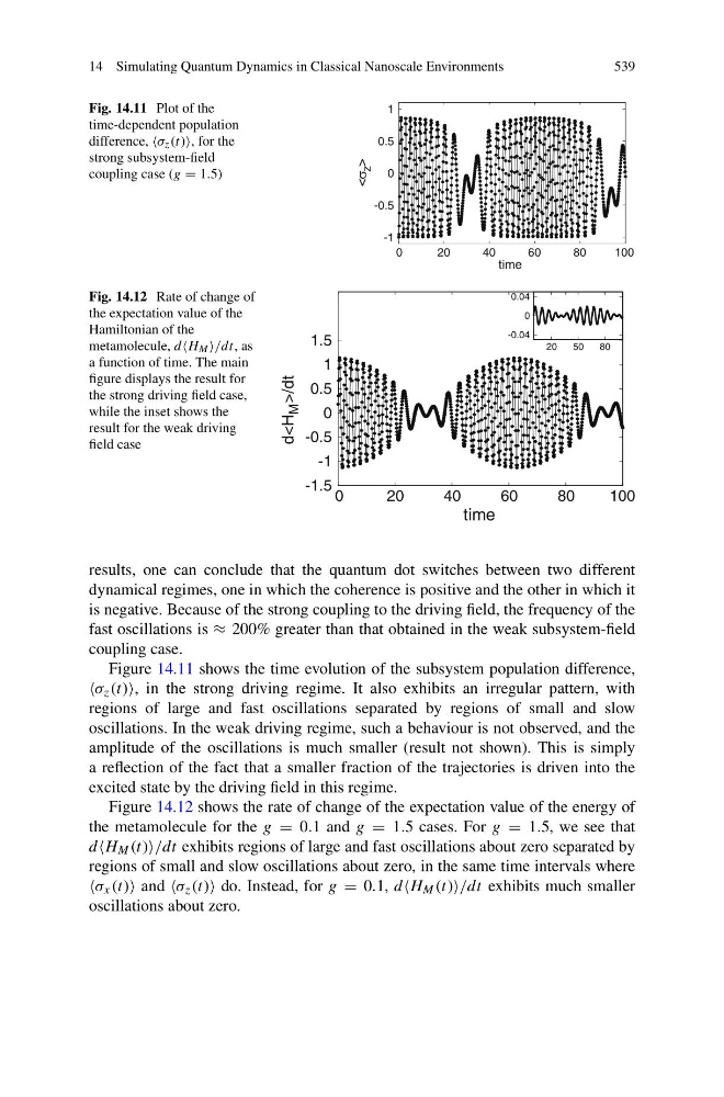
Fig. 14.11 Plot of the
time-dependent population
difference, σ z (t), for the
strong subsystem-field
coupling case (g = 1.5)
-1
-0.5
0
0.5
1
0
20
40
60
80
100
<σ
z >
time
Fig. 14.12 Rate of change of
the expectation value of the
Hamiltonian of the
metamolecule, dH M /dt, as
a function of time. The main
figure displays the result for
the strong driving field case,
while the inset shows the
result for the weak driving
field case
-1.5
-1
-0.5
0
0.5
1
1.5
0
20
40
60
80
100
d M >/dt
time
-0.04
0
0.04
20
50
80
results, one can conclude that the quantum dot switches between two different
dynamical regimes, one in which the coherence is positive and the other in which it
is negative. Because of the strong coupling to the driving field, the frequency of the
fast oscillations is ≈ 200% greater than that obtained in the weak subsystem-field
coupling case.
Figure 14.11 shows the time evolution of the subsystem population difference,
σ z (t), in the strong driving regime. It also exhibits an irregular pattern, with
regions of large and fast oscillations separated by regions of small and slow
oscillations. In the weak driving regime, such a behaviour is not observed, and the
amplitude of the oscillations is much smaller (result not shown). This is simply
a reflection of the fact that a smaller fraction of the trajectories is driven into the
excited state by the driving field in this regime.
Figure 14.12 shows the rate of change of the expectation value of the energy of
the metamolecule for the g = 0.1 and g = 1.5 cases. For g = 1.5, we see that
dH M (t)/dt exhibits regions of large and fast oscillations about zero separated by
regions of small and slow oscillations about zero, in the same time intervals where
σ x (t) and σ z (t) do. Instead, for g = 0.1, dH M (t)/dt exhibits much smaller
oscillations about zero.