

14 Simulating Quantum Dynamics in Classical Nanoscale Environments
537
˜
T
∗
α →β (t) =
P
M
· d
∗
α β (Q, t)
1 +
1
2
E α β (t)d ∗
α β (Q, t)
P
M · d ∗
αβ (Q, t)
∂
∂P
, (14.42)
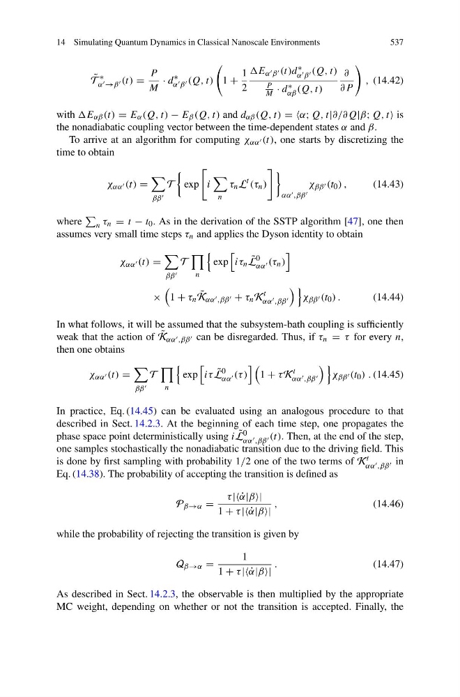
with E αβ (t) = E α (Q, t) − E β (Q, t) and d αβ (Q, t) = =α; Q, t|∂/∂Q|β; Q, t is
the nonadiabatic coupling vector between the time-dependent states α and β.
To arrive at an algorithm for computing χ αα (t), one starts by discretizing the
time to obtain
χ αα (t) =
ββ
T
exp
i
n
τ n L
t (τ n )
αα ,ββ
χ ββ (t 0 ) ,
(14.43)
where
n τ n = t − t 0 . As in the derivation of the SSTP algorithm [47], one then
assumes very small time steps τ n and applies the Dyson identity to obtain
χ αα (t) =
ββ
T
n
exp
iτ n ˜
L
0
αα (τ n )
×
1 + τ n ˜
K αα ,ββ + τ n K
t
αα ,ββ
χ ββ (t 0 ) .
(14.44)
In what follows, it will be assumed that the subsystem-bath coupling is sufficiently
weak that the action of ˜
K αα ,ββ can be disregarded. Thus, if τ n = τ for every n,
then one obtains
χ αα (t) =
ββ
T
n
exp
iτ ˜
L
0
αα (τ )
1 + τ K
t
αα ,ββ
χ ββ (t 0 ) . (14.45)
In practice, Eq. (14.45) can be evaluated using an analogous procedure to that
described in Sect. 14.2.3. At the beginning of each time step, one propagates the
phase space point deterministically using i ˜
L 0
αα ,ββ (t). Then, at the end of the step,
one samples stochastically the nonadiabatic transition due to the driving field. This
is done by first sampling with probability 1/2 one of the two terms of K t
αα ,ββ in
Eq. (14.38). The probability of accepting the transition is defined as
P β→α =
τ || ˙
α|β|
1 + τ || ˙
α|β|
,
(14.46)
while the probability of rejecting the transition is given by
Q β→α =
1
1 + τ || ˙
α|β|
.
(14.47)
As described in Sect. 14.2.3, the observable is then multiplied by the appropriate
MC weight, depending on whether or not the transition is accepted. Finally, the
537
˜
T
∗
α →β (t) =
P
M
· d
∗
α β (Q, t)
1 +
1
2
E α β (t)d ∗
α β (Q, t)
P
M · d ∗
αβ (Q, t)
∂
∂P
, (14.42)
with E αβ (t) = E α (Q, t) − E β (Q, t) and d αβ (Q, t) = =α; Q, t|∂/∂Q|β; Q, t is
the nonadiabatic coupling vector between the time-dependent states α and β.
To arrive at an algorithm for computing χ αα (t), one starts by discretizing the
time to obtain
χ αα (t) =
ββ
T
exp
i
n
τ n L
t (τ n )
αα ,ββ
χ ββ (t 0 ) ,
(14.43)
where
n τ n = t − t 0 . As in the derivation of the SSTP algorithm [47], one then
assumes very small time steps τ n and applies the Dyson identity to obtain
χ αα (t) =
ββ
T
n
exp
iτ n ˜
L
0
αα (τ n )
×
1 + τ n ˜
K αα ,ββ + τ n K
t
αα ,ββ
χ ββ (t 0 ) .
(14.44)
In what follows, it will be assumed that the subsystem-bath coupling is sufficiently
weak that the action of ˜
K αα ,ββ can be disregarded. Thus, if τ n = τ for every n,
then one obtains
χ αα (t) =
ββ
T
n
exp
iτ ˜
L
0
αα (τ )
1 + τ K
t
αα ,ββ
χ ββ (t 0 ) . (14.45)
In practice, Eq. (14.45) can be evaluated using an analogous procedure to that
described in Sect. 14.2.3. At the beginning of each time step, one propagates the
phase space point deterministically using i ˜
L 0
αα ,ββ (t). Then, at the end of the step,
one samples stochastically the nonadiabatic transition due to the driving field. This
is done by first sampling with probability 1/2 one of the two terms of K t
αα ,ββ in
Eq. (14.38). The probability of accepting the transition is defined as
P β→α =
τ || ˙
α|β|
1 + τ || ˙
α|β|
,
(14.46)
while the probability of rejecting the transition is given by
Q β→α =
1
1 + τ || ˙
α|β|
.
(14.47)
As described in Sect. 14.2.3, the observable is then multiplied by the appropriate
MC weight, depending on whether or not the transition is accepted. Finally, the