

14 Simulating Quantum Dynamics in Classical Nanoscale Environments
533
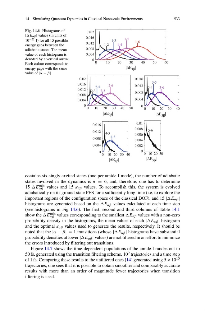
Fig. 14.6 Histograms of
|E αβ | values (in units of
10 −22 J) for all 15 possible
energy gaps between the
adiabatic states. The mean
value of each histogram is
denoted by a vertical arrow.
Each colour corresponds to
energy gaps with the same
value of |α − β|
contains six singly excited states (one per amide I mode), the number of adiabatic
states involved in the dynamics is n = 6, and, therefore, one has to determine
15 E min
αβ values and 15 κ αβ values. To accomplish this, the system is evolved
adiabatically on its ground-state PES for a sufficiently long time (i.e. to explore the
important regions of the configuration space of the classical DOF), and 15 |E αβ |
histograms are generated based on the E αβ values calculated at each time step
(see histograms in Fig. 14.6). The first, second and third columns of Table 14.1
show the E min
αβ values corresponding to the smallest E αβ values with a non-zero
probability density in the histograms, the mean values of each |E αβ | histogram
and the optimal κ αβ values used to generate the results, respectively. It should be
noted that the |α − β| = 1 transitions (whose |E αβ | histograms have substantial
probability densities at lower |E αβ | values) are not filtered in an effort to minimize
the errors introduced by filtering out transitions.
Figure 14.7 shows the time-dependent populations of the amide I modes out to
50 fs, generated using the transition filtering scheme, 10 9 trajectories and a time step
of 1 fs. Comparing these results to the unfiltered ones [14] generated using 5 × 10 10
trajectories, one sees that it is possible to obtain smoother and comparably accurate
results with more than an order of magnitude fewer trajectories when transition
filtering is used.
533
Fig. 14.6 Histograms of
|E αβ | values (in units of
10 −22 J) for all 15 possible
energy gaps between the
adiabatic states. The mean
value of each histogram is
denoted by a vertical arrow.
Each colour corresponds to
energy gaps with the same
value of |α − β|
contains six singly excited states (one per amide I mode), the number of adiabatic
states involved in the dynamics is n = 6, and, therefore, one has to determine
15 E min
αβ values and 15 κ αβ values. To accomplish this, the system is evolved
adiabatically on its ground-state PES for a sufficiently long time (i.e. to explore the
important regions of the configuration space of the classical DOF), and 15 |E αβ |
histograms are generated based on the E αβ values calculated at each time step
(see histograms in Fig. 14.6). The first, second and third columns of Table 14.1
show the E min
αβ values corresponding to the smallest E αβ values with a non-zero
probability density in the histograms, the mean values of each |E αβ | histogram
and the optimal κ αβ values used to generate the results, respectively. It should be
noted that the |α − β| = 1 transitions (whose |E αβ | histograms have substantial
probability densities at lower |E αβ | values) are not filtered in an effort to minimize
the errors introduced by filtering out transitions.
Figure 14.7 shows the time-dependent populations of the amide I modes out to
50 fs, generated using the transition filtering scheme, 10 9 trajectories and a time step
of 1 fs. Comparing these results to the unfiltered ones [14] generated using 5 × 10 10
trajectories, one sees that it is possible to obtain smoother and comparably accurate
results with more than an order of magnitude fewer trajectories when transition
filtering is used.