

14 Simulating Quantum Dynamics in Classical Nanoscale Environments
521
ˆ
χ(t) = Tr
dQdP ˆ
ρ(Q, P ) ˆ
χ(Q, P , t) ,
(14.4)
where the mixed quantum-classical equation of motion of ˆ
χ(Q, P , t) is given by
∂
∂t
ˆ
χ(Q, P , t) =
i
¯
h
ˆ
H , ˆ
χ(Q, P , t)
−
1
2
ˆ
H , ˆ
χ(Q, P , t)
+
1
2
ˆ
χ(Q, P , t), ˆ
H
.
(14.5)
14.2.2 Representing the QCLE in the Adiabatic Basis
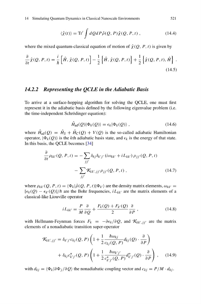
To arrive at a surface-hopping algorithm for solving the QCLE, one must first
represent it in the adiabatic basis defined by the following eigenvalue problem (i.e.
the time-independent Schrödinger equation):
ˆ
H ad (Q)| k (Q) = k | k (Q) ,
(14.6)
where ˆ
H ad (Q) = ˆ
H S + ˆ
H C (Q) + V (Q) is the so-called adiabatic Hamiltonian
operator, | k (Q) is the kth adiabatic basis state, and k is the energy of that state.
In this basis, the QCLE becomes [34]
∂
∂t
ρ kk (Q, P , t) = −
jj
δ kj δ k j (iω kk + iL kk ) ρ jj (Q, P , t)
−
jj
K kk ,jj ρ jj (Q, P , t) ,
(14.7)
where ρ kk (Q, P , t) = = k | ˆ
ρ(Q, P , t)| k are the density matrix elements, ω kk =
[ k (Q) − k (Q)]/ ¯
h are the Bohr frequencies, iL kk are the matrix elements of a
classical-like Liouville operator
iL kk =
P
M
∂
∂Q
+
F k (Q) + F k (Q)
2
∂
∂P
,
(14.8)
with Hellmann-Feynman forces F k = −∂∂ k /∂Q, and K kk ,jj are the matrix
elements of a nonadiabatic transition super-operator
K kk ,jj = δ k j c kj (Q, P )
1 +
1
2
¯
hω kj
c kj (Q, P )
d kj (Q) ·
∂
∂P
+ δ kj c
∗
k j (Q, P )
1 +
1
2
¯
hω k j
c ∗
k j (Q, P )
d
∗
k j (Q) ·
∂
∂P
,
(14.9)
with d kj = = k |∂∂ j /∂Q the nonadiabatic coupling vector and c kj = P /M · d kj .
521
ˆ
χ(t) = Tr
dQdP ˆ
ρ(Q, P ) ˆ
χ(Q, P , t) ,
(14.4)
where the mixed quantum-classical equation of motion of ˆ
χ(Q, P , t) is given by
∂
∂t
ˆ
χ(Q, P , t) =
i
¯
h
ˆ
H , ˆ
χ(Q, P , t)
−
1
2
ˆ
H , ˆ
χ(Q, P , t)
+
1
2
ˆ
χ(Q, P , t), ˆ
H
.
(14.5)
14.2.2 Representing the QCLE in the Adiabatic Basis
To arrive at a surface-hopping algorithm for solving the QCLE, one must first
represent it in the adiabatic basis defined by the following eigenvalue problem (i.e.
the time-independent Schrödinger equation):
ˆ
H ad (Q)| k (Q) = k | k (Q) ,
(14.6)
where ˆ
H ad (Q) = ˆ
H S + ˆ
H C (Q) + V (Q) is the so-called adiabatic Hamiltonian
operator, | k (Q) is the kth adiabatic basis state, and k is the energy of that state.
In this basis, the QCLE becomes [34]
∂
∂t
ρ kk (Q, P , t) = −
jj
δ kj δ k j (iω kk + iL kk ) ρ jj (Q, P , t)
−
jj
K kk ,jj ρ jj (Q, P , t) ,
(14.7)
where ρ kk (Q, P , t) = = k | ˆ
ρ(Q, P , t)| k are the density matrix elements, ω kk =
[ k (Q) − k (Q)]/ ¯
h are the Bohr frequencies, iL kk are the matrix elements of a
classical-like Liouville operator
iL kk =
P
M
∂
∂Q
+
F k (Q) + F k (Q)
2
∂
∂P
,
(14.8)
with Hellmann-Feynman forces F k = −∂∂ k /∂Q, and K kk ,jj are the matrix
elements of a nonadiabatic transition super-operator
K kk ,jj = δ k j c kj (Q, P )
1 +
1
2
¯
hω kj
c kj (Q, P )
d kj (Q) ·
∂
∂P
+ δ kj c
∗
k j (Q, P )
1 +
1
2
¯
hω k j
c ∗
k j (Q, P )
d
∗
k j (Q) ·
∂
∂P
,
(14.9)
with d kj = = k |∂∂ j /∂Q the nonadiabatic coupling vector and c kj = P /M · d kj .