

522
G. Hanna and A. Sergi
14.2.3 The Sequential Short-Time Propagation Algorithm
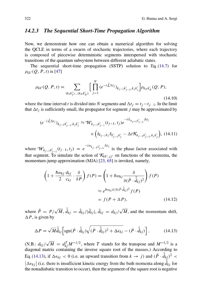
Now, we demonstrate how one can obtain a numerical algorithm for solving
the QCLE in terms of a swarm of stochastic trajectories, where each trajectory
is composed of piecewise deterministic segments interspersed with stochastic
transitions of the quantum subsystem between different adiabatic states.
The sequential short-time propagation (SSTP) solution to Eq. (14.7) for
ρ kk (Q, P , t) is [47]
ρ kk (Q, P , t) =
(k 1 k
1 )...(k N k
N )
N
j =1
(e
−i ˆ
Lt j ) k j −1 k
j −1 ,k j k
j
ρ k N k
N
(Q, P ),
(14.10)
where the time interval t is divided into N segments and t j = t j −t j −1 . In the limit
that t j is sufficiently small, the propagator for segment j may be approximated by
(e
−i ˆ
Lt j ) k j −1 k
j −1 ,k j k
j
≈ W k j −1 k
j −1
(t j −1 , t j )e
−iL k j −1 k
j −1
t j
×
δ k j −1 k j δ k
j −1 k
j
− tK k j −1 k
j −1 ,k j k
j
, (14.11)
where W k j −1 k
j −1
(t j −1 , t j ) = e
−iω k j −1 k
j −1
t j is the phase factor associated with
that segment. To simulate the action of K kk ,jj on functions of the momenta, the
momentum-jump approximation (MJA) [23, 65] is invoked, namely,
1 +
¯
hω kj
2
d kj
c kj
·
∂
∂P
f (P ) =
1 + ¯
hω kj
∂
∂( ¯
P · ¯ ˆ
d kj ) 2
f (P )
≈ e ¯
hω kj ∂/∂( ¯
P · ¯ ˆ
d kj ) 2 f (P )
= f (P + P ),
(14.12)
where ¯
P = P /
√
M, ¯ ˆ
d kj = ¯
d kj /| ¯
d kj |, ¯
d kj = d kj /
√
M, and the momentum shift,
P , is given by
P =
√
M ¯ ˆ
d kj
sgn( ¯
P · ¯ ˆ
d kj )
( ¯
P · ¯ ˆ
d kj ) 2 + kj − ( ¯
P · ¯ ˆ
d kj )
.
(14.13)
(N.B.: d kj /
√
M = d T
kj M −1/2 , where T stands for the transpose and M −1/2 is a
diagonal matrix containing the inverse square root of the masses.) According to
Eq. (14.13), if kj < 0 (i.e. an upward transition from k → j) and ( ¯
P · ¯ ˆ
d kj ) 2 <
kj
(i.e. there is insufficient kinetic energy from the bath momenta along ¯ ˆ
d kj for
the nonadiabatic transition to occur), then the argument of the square root is negative
G. Hanna and A. Sergi
14.2.3 The Sequential Short-Time Propagation Algorithm
Now, we demonstrate how one can obtain a numerical algorithm for solving
the QCLE in terms of a swarm of stochastic trajectories, where each trajectory
is composed of piecewise deterministic segments interspersed with stochastic
transitions of the quantum subsystem between different adiabatic states.
The sequential short-time propagation (SSTP) solution to Eq. (14.7) for
ρ kk (Q, P , t) is [47]
ρ kk (Q, P , t) =
(k 1 k
1 )...(k N k
N )
N
j =1
(e
−i ˆ
Lt j ) k j −1 k
j −1 ,k j k
j
ρ k N k
N
(Q, P ),
(14.10)
where the time interval t is divided into N segments and t j = t j −t j −1 . In the limit
that t j is sufficiently small, the propagator for segment j may be approximated by
(e
−i ˆ
Lt j ) k j −1 k
j −1 ,k j k
j
≈ W k j −1 k
j −1
(t j −1 , t j )e
−iL k j −1 k
j −1
t j
×
δ k j −1 k j δ k
j −1 k
j
− tK k j −1 k
j −1 ,k j k
j
, (14.11)
where W k j −1 k
j −1
(t j −1 , t j ) = e
−iω k j −1 k
j −1
t j is the phase factor associated with
that segment. To simulate the action of K kk ,jj on functions of the momenta, the
momentum-jump approximation (MJA) [23, 65] is invoked, namely,
1 +
¯
hω kj
2
d kj
c kj
·
∂
∂P
f (P ) =
1 + ¯
hω kj
∂
∂( ¯
P · ¯ ˆ
d kj ) 2
f (P )
≈ e ¯
hω kj ∂/∂( ¯
P · ¯ ˆ
d kj ) 2 f (P )
= f (P + P ),
(14.12)
where ¯
P = P /
√
M, ¯ ˆ
d kj = ¯
d kj /| ¯
d kj |, ¯
d kj = d kj /
√
M, and the momentum shift,
P , is given by
P =
√
M ¯ ˆ
d kj
sgn( ¯
P · ¯ ˆ
d kj )
( ¯
P · ¯ ˆ
d kj ) 2 + kj − ( ¯
P · ¯ ˆ
d kj )
.
(14.13)
(N.B.: d kj /
√
M = d T
kj M −1/2 , where T stands for the transpose and M −1/2 is a
diagonal matrix containing the inverse square root of the masses.) According to
Eq. (14.13), if kj < 0 (i.e. an upward transition from k → j) and ( ¯
P · ¯ ˆ
d kj ) 2 <
kj
(i.e. there is insufficient kinetic energy from the bath momenta along ¯ ˆ
d kj for
the nonadiabatic transition to occur), then the argument of the square root is negative