

520
G. Hanna and A. Sergi
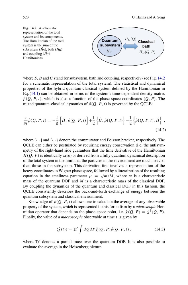
Fig. 14.2 A schematic
representation of the total
system and its components.
The Hamiltonian of the total
system is the sum of the
subsystem ( ˆ
H S ), bath (H B )
and coupling ( ˆ
H C )
Hamiltonians
Classical
bath
Quantum
subsystem
ˆ
H S
H B (Q, P )
ˆ
H C (Q)
where S, B and C stand for subsystem, bath and coupling, respectively (see Fig. 14.2
for a schematic representation of the total system). The statistical and dynamical
properties of the hybrid quantum-classical system defined by the Hamiltonian in
Eq. (14.1) can be obtained in terms of the system’s time-dependent density matrix
ˆ
ρ(Q, P , t), which is also a function of the phase space coordinates (Q, P ). The
mixed quantum-classical dynamics of ˆ
ρ(Q, P , t) is governed by the QCLE:
∂
∂t
ˆ
ρ(Q, P , t) = −
i
¯
h
ˆ
H , ˆ
ρ(Q, P , t)
+
1
2
ˆ
H , ˆ
ρ(Q, P , t)
−
1
2
ˆ
ρ(Q, P , t), ˆ
H
,
(14.2)
where [·, ·] and {·, ·} denote the commutator and Poisson bracket, respectively. The
QCLE can either be postulated by requiring energy conservation (i.e. the antisymmetry of the right-hand side guarantees that the time derivative of the Hamiltonian
ˆ
H (Q, P ) is identically zero) or derived from a fully quantum dynamical description
of the total system in the limit that the particles in the environment are much heavier
than those in the subsystem. This derivation first involves a representation of the
heavy coordinates in Wigner phase space, followed by a linearization of the resulting
equation in the smallness parameter μ =
√
m/M, where m is a characteristic
mass of the quantum DOF and M is a characteristic mass of the classical DOF.
By coupling the dynamics of the quantum and classical DOF in this fashion, the
QCLE consistently describes the back-and-forth exchange of energy between the
quantum subsystem and classical environment.
Knowledge of ˆ
ρ(Q, P , t) allows one to calculate the average of any observable
property of the system, which is represented in this formalism by a microscopic Hermitian operator that depends on the phase space point, i.e. ˆ
χ(Q, P ) = ˆ
χ † (Q, P ).
Finally, the value of a macroscopic observable at time t is given by
ˆ
χ(t) = Tr
dQdP ˆ
χ(Q, P ) ˆ
ρ(Q, P , t) ,
(14.3)
where Tr denotes a partial trace over the quantum DOF. It is also possible to
evaluate the average in the Heisenberg picture,
G. Hanna and A. Sergi
Fig. 14.2 A schematic
representation of the total
system and its components.
The Hamiltonian of the total
system is the sum of the
subsystem ( ˆ
H S ), bath (H B )
and coupling ( ˆ
H C )
Hamiltonians
Classical
bath
Quantum
subsystem
ˆ
H S
H B (Q, P )
ˆ
H C (Q)
where S, B and C stand for subsystem, bath and coupling, respectively (see Fig. 14.2
for a schematic representation of the total system). The statistical and dynamical
properties of the hybrid quantum-classical system defined by the Hamiltonian in
Eq. (14.1) can be obtained in terms of the system’s time-dependent density matrix
ˆ
ρ(Q, P , t), which is also a function of the phase space coordinates (Q, P ). The
mixed quantum-classical dynamics of ˆ
ρ(Q, P , t) is governed by the QCLE:
∂
∂t
ˆ
ρ(Q, P , t) = −
i
¯
h
ˆ
H , ˆ
ρ(Q, P , t)
+
1
2
ˆ
H , ˆ
ρ(Q, P , t)
−
1
2
ˆ
ρ(Q, P , t), ˆ
H
,
(14.2)
where [·, ·] and {·, ·} denote the commutator and Poisson bracket, respectively. The
QCLE can either be postulated by requiring energy conservation (i.e. the antisymmetry of the right-hand side guarantees that the time derivative of the Hamiltonian
ˆ
H (Q, P ) is identically zero) or derived from a fully quantum dynamical description
of the total system in the limit that the particles in the environment are much heavier
than those in the subsystem. This derivation first involves a representation of the
heavy coordinates in Wigner phase space, followed by a linearization of the resulting
equation in the smallness parameter μ =
√
m/M, where m is a characteristic
mass of the quantum DOF and M is a characteristic mass of the classical DOF.
By coupling the dynamics of the quantum and classical DOF in this fashion, the
QCLE consistently describes the back-and-forth exchange of energy between the
quantum subsystem and classical environment.
Knowledge of ˆ
ρ(Q, P , t) allows one to calculate the average of any observable
property of the system, which is represented in this formalism by a microscopic Hermitian operator that depends on the phase space point, i.e. ˆ
χ(Q, P ) = ˆ
χ † (Q, P ).
Finally, the value of a macroscopic observable at time t is given by
ˆ
χ(t) = Tr
dQdP ˆ
χ(Q, P ) ˆ
ρ(Q, P , t) ,
(14.3)
where Tr denotes a partial trace over the quantum DOF. It is also possible to
evaluate the average in the Heisenberg picture,