

492
N. C. Bacalis
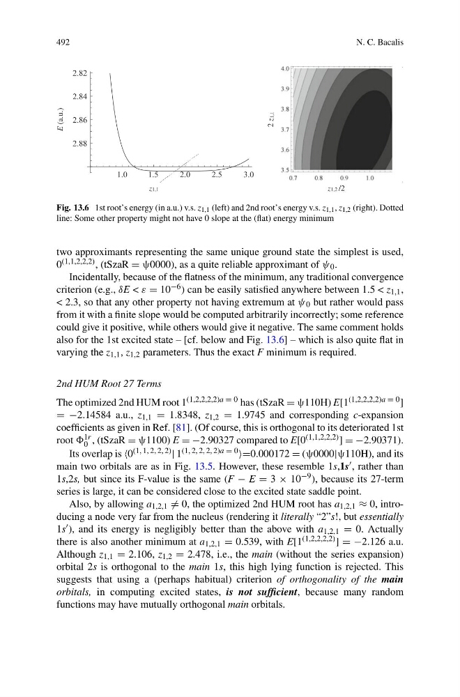
Fig. 13.6 1st root’s energy (in a.u.) v.s. z 1,1 (left) and 2nd root’s energy v.s. z 1,1 , z 1,2 (right). Dotted
line: Some other property might not have 0 slope at the (flat) energy minimum
two approximants representing the same unique ground state the simplest is used,
0 (1,1,2,2,2) , (tSzaR = ψ0000), as a quite reliable approximant of ψ 0 .
Incidentally, because of the flatness of the minimum, any traditional convergence
criterion (e.g., δE < ε = 10 −6 ) can be easily satisfied anywhere between 1.5 < z 1,1 ,
< 2.3, so that any other property not having extremum at ψ 0 but rather would pass
from it with a finite slope would be computed arbitrarily incorrectly; some reference
could give it positive, while others would give it negative. The same comment holds
also for the 1st excited state – [cf. below and Fig. 13.6] – which is also quite flat in
varying the z 1,1 , z 1,2 parameters. Thus the exact F minimum is required.
2nd HUM Root 27 Terms
The optimized 2nd HUM root 1 (1,2,2,2,2)a = 0 has (tSzaR = ψ110H) E[1 (1,2,2,2,2)a = 0 ]
= −2.14584 a.u., z 1,1 = 1.8348, z 1,2 = 1.9745 and corresponding c-expansion
coefficients as given in Ref. [81]. (Of course, this is orthogonal to its deteriorated 1st
root 1r
0 , (tSzaR = ψ1100) E = −2.90327 compared to E[0 (1,1,2,2,2) ] = −2.90371).
Its overlap is 0 (1, 1, 2, 2, 2) | 1 (1, 2, 2, 2, 2)a = 0 =0.000172 = (ψ0000|ψ110H), and its
main two orbitals are as in Fig. 13.5. However, these resemble 1s,1s , rather than
1s,2s, but since its F-value is the same (F − E = 3 × 10 −9 ), because its 27-term
series is large, it can be considered close to the excited state saddle point.
Also, by allowing a 1,2,1 = 0, the optimized 2nd HUM root has a 1,2,1 ≈ 0, introducing a node very far from the nucleus (rendering it literally “2”s!, but essentially
1s ), and its energy is negligibly better than the above with a 1,2,1 = 0. Actually
there is also another minimum at a 1,2,1 = 0.539, with E[1 (1,2,2,2,2) ] = −2.126 a.u.
Although z 1,1 = 2.106, z 1,2 = 2.478, i.e., the main (without the series expansion)
orbital 2s is orthogonal to the main 1s, this high lying function is rejected. This
suggests that using a (perhaps habitual) criterion of orthogonality of the main
orbitals, in computing excited states, is not sufficient, because many random
functions may have mutually orthogonal main orbitals.
N. C. Bacalis
Fig. 13.6 1st root’s energy (in a.u.) v.s. z 1,1 (left) and 2nd root’s energy v.s. z 1,1 , z 1,2 (right). Dotted
line: Some other property might not have 0 slope at the (flat) energy minimum
two approximants representing the same unique ground state the simplest is used,
0 (1,1,2,2,2) , (tSzaR = ψ0000), as a quite reliable approximant of ψ 0 .
Incidentally, because of the flatness of the minimum, any traditional convergence
criterion (e.g., δE < ε = 10 −6 ) can be easily satisfied anywhere between 1.5 < z 1,1 ,
< 2.3, so that any other property not having extremum at ψ 0 but rather would pass
from it with a finite slope would be computed arbitrarily incorrectly; some reference
could give it positive, while others would give it negative. The same comment holds
also for the 1st excited state – [cf. below and Fig. 13.6] – which is also quite flat in
varying the z 1,1 , z 1,2 parameters. Thus the exact F minimum is required.
2nd HUM Root 27 Terms
The optimized 2nd HUM root 1 (1,2,2,2,2)a = 0 has (tSzaR = ψ110H) E[1 (1,2,2,2,2)a = 0 ]
= −2.14584 a.u., z 1,1 = 1.8348, z 1,2 = 1.9745 and corresponding c-expansion
coefficients as given in Ref. [81]. (Of course, this is orthogonal to its deteriorated 1st
root 1r
0 , (tSzaR = ψ1100) E = −2.90327 compared to E[0 (1,1,2,2,2) ] = −2.90371).
Its overlap is 0 (1, 1, 2, 2, 2) | 1 (1, 2, 2, 2, 2)a = 0 =0.000172 = (ψ0000|ψ110H), and its
main two orbitals are as in Fig. 13.5. However, these resemble 1s,1s , rather than
1s,2s, but since its F-value is the same (F − E = 3 × 10 −9 ), because its 27-term
series is large, it can be considered close to the excited state saddle point.
Also, by allowing a 1,2,1 = 0, the optimized 2nd HUM root has a 1,2,1 ≈ 0, introducing a node very far from the nucleus (rendering it literally “2”s!, but essentially
1s ), and its energy is negligibly better than the above with a 1,2,1 = 0. Actually
there is also another minimum at a 1,2,1 = 0.539, with E[1 (1,2,2,2,2) ] = −2.126 a.u.
Although z 1,1 = 2.106, z 1,2 = 2.478, i.e., the main (without the series expansion)
orbital 2s is orthogonal to the main 1s, this high lying function is rejected. This
suggests that using a (perhaps habitual) criterion of orthogonality of the main
orbitals, in computing excited states, is not sufficient, because many random
functions may have mutually orthogonal main orbitals.