

13 If Truncated Wave Functions of Excited State Energy Saddle Points Are. . .
493
Schr (a.u.)
1.55
1.60
1.65
1.70
1.75
1.80
–0.0005
0.0005
0.0010
0.0015
a
b
d
c
z 0
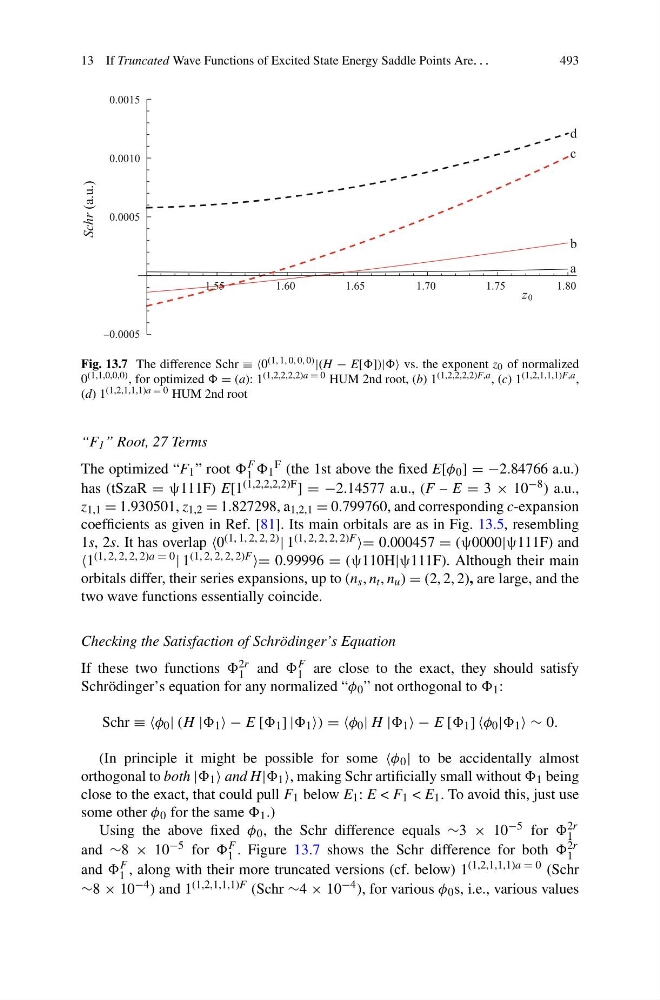
Fig. 13.7 The difference Schr ≡ ≡0 (1, 1, 0, 0, 0) |(H − E[])| vs. the exponent z 0 of normalized
0 (1,1,0,0,0) , for optimized = (a): 1 (1,2,2,2,2)a = 0 HUM 2nd root, (b) 1 (1,2,2,2,2)F,a , (c) 1 (1,2,1,1,1)F,a ,
(d) 1 (1,2,1,1,1)a = 0 HUM 2nd root
“F 1 ” Root, 27 Terms
The optimized “F 1 ” root F
1 1
F (the 1st above the fixed E[φ 0 ] = −2.84766 a.u.)
has (tSzaR = ψ111F) E[1 (1,2,2,2,2)F ] = −2.14577 a.u., (F – E = 3 × 10 −8 ) a.u.,
z 1,1 = 1.930501, z 1,2 = 1.827298, a 1,2,1 = 0.799760, and corresponding c-expansion
coefficients as given in Ref. [81]. Its main orbitals are as in Fig. 13.5, resembling
1s, 2s. It has overlap 0 (1, 1, 2, 2, 2) | 1 (1, 2, 2, 2, 2)F = 0.000457 = (ψ0000|ψ111F) and
1 (1, 2, 2, 2, 2)a = 0 | 1 (1, 2, 2, 2, 2)F = 0.99996 = (ψ110H|ψ111F). Although their main
orbitals differ, their series expansions, up to (n s , n t , n u ) = (2, 2, 2), are large, and the
two wave functions essentially coincide.
Checking the Satisfaction of Schrödinger’s Equation
If these two functions 2r
1 and F
1 are close to the exact, they should satisfy
Schrödinger’s equation for any normalized “φ 0 ” not orthogonal to 1 :
Schr ≡ φ 0 | (H | 1 − E [ 1 ] | 1 ) = φ 0 | H | 1 − E [ 1 ] φ 0 | 1 ∼ 0.
(In principle it might be possible for some φ 0 | to be accidentally almost
orthogonal to both | 1 and H| 1 , making Schr artificially small without 1 being
close to the exact, that could pull F 1 below E 1 : E < F 1 < E 1 . To avoid this, just use
some other φ 0 for the same 1 .)
Using the above fixed φ 0 , the Schr difference equals ∼3 × 10 −5 for 2r
1
and ∼8 × 10 −5 for F
1 . Figure 13.7 shows the Schr difference for both 2r
1
and F
1 , along with their more truncated versions (cf. below) 1 (1,2,1,1,1)a = 0 (Schr
∼8 × 10 −4 ) and 1 (1,2,1,1,1)F (Schr ∼4 × 10 −4 ), for various φ 0 s, i.e., various values
493
Schr (a.u.)
1.55
1.60
1.65
1.70
1.75
1.80
–0.0005
0.0005
0.0010
0.0015
a
b
d
c
z 0
Fig. 13.7 The difference Schr ≡ ≡0 (1, 1, 0, 0, 0) |(H − E[])| vs. the exponent z 0 of normalized
0 (1,1,0,0,0) , for optimized = (a): 1 (1,2,2,2,2)a = 0 HUM 2nd root, (b) 1 (1,2,2,2,2)F,a , (c) 1 (1,2,1,1,1)F,a ,
(d) 1 (1,2,1,1,1)a = 0 HUM 2nd root
“F 1 ” Root, 27 Terms
The optimized “F 1 ” root F
1 1
F (the 1st above the fixed E[φ 0 ] = −2.84766 a.u.)
has (tSzaR = ψ111F) E[1 (1,2,2,2,2)F ] = −2.14577 a.u., (F – E = 3 × 10 −8 ) a.u.,
z 1,1 = 1.930501, z 1,2 = 1.827298, a 1,2,1 = 0.799760, and corresponding c-expansion
coefficients as given in Ref. [81]. Its main orbitals are as in Fig. 13.5, resembling
1s, 2s. It has overlap 0 (1, 1, 2, 2, 2) | 1 (1, 2, 2, 2, 2)F = 0.000457 = (ψ0000|ψ111F) and
1 (1, 2, 2, 2, 2)a = 0 | 1 (1, 2, 2, 2, 2)F = 0.99996 = (ψ110H|ψ111F). Although their main
orbitals differ, their series expansions, up to (n s , n t , n u ) = (2, 2, 2), are large, and the
two wave functions essentially coincide.
Checking the Satisfaction of Schrödinger’s Equation
If these two functions 2r
1 and F
1 are close to the exact, they should satisfy
Schrödinger’s equation for any normalized “φ 0 ” not orthogonal to 1 :
Schr ≡ φ 0 | (H | 1 − E [ 1 ] | 1 ) = φ 0 | H | 1 − E [ 1 ] φ 0 | 1 ∼ 0.
(In principle it might be possible for some φ 0 | to be accidentally almost
orthogonal to both | 1 and H| 1 , making Schr artificially small without 1 being
close to the exact, that could pull F 1 below E 1 : E < F 1 < E 1 . To avoid this, just use
some other φ 0 for the same 1 .)
Using the above fixed φ 0 , the Schr difference equals ∼3 × 10 −5 for 2r
1
and ∼8 × 10 −5 for F
1 . Figure 13.7 shows the Schr difference for both 2r
1
and F
1 , along with their more truncated versions (cf. below) 1 (1,2,1,1,1)a = 0 (Schr
∼8 × 10 −4 ) and 1 (1,2,1,1,1)F (Schr ∼4 × 10 −4 ), for various φ 0 s, i.e., various values