

486
N. C. Bacalis
In the next section, the formalism will be described (see [81] for matrix elements
of φ i | φ n , φ i |H|φ n in Hylleraas coordinates). Then, the results will be presented,
including the immediate improvement of φ 0 via a more accurate φ 1 . And then, a
demonstration of recognizing a “flipped root” near the crossing will follow. After
the demonstrations using the Hylleraas coordinates demonstrations for He and Li
by conventional CI computation, appropriate for any number of electrons, will be
presented.
13.6.1 Formalism in Hylleraas Coordinates
For two-electron atomic ions of nuclear charge Z, the wave function will consist of
a single Slater determinant multiplied by a truncated power series of s = r 1 + r 2 ,
t = r 1 − r 2 , and u =
− → r 1 − − → r 2
:
n s ,n t ,n u
i s ,i t ,i u =0
c i s ,i t ,i u s i s t 2i t u i u . Due to the spin
antisymmetry, the Slater determinant is reduced to a symmetric sum of products and
the power series to a symmetric function of t, i.e., of t 2 . And since the Hamiltonian
is also symmetric, the t-integrals could be evaluated only for t > 0 (eventually
multiplied by 2), so that, with volume element 2π 2 (s 2 − t 2 )u dt du ds, the limits
of integration be 0 < t ≤ u ≤ s < ∞ [82].
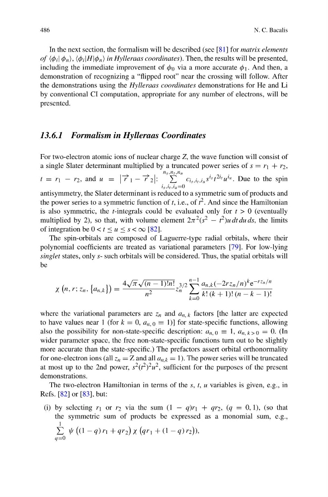
The spin-orbitals are composed of Laguerre-type radial orbitals, where their
polynomial coefficients are treated as variational parameters [79]. For low-lying
singlet states, only s- such orbitals will be considered. Thus, the spatial orbitals will
be
χ
n, r; z n ,
a n,k
=
4
√
π
√
(n − 1)!n!
n 2
z
3/2
n
n−1
k=0
a n,k (−2rz n /n)
k e −rz n /n
k! (k + 1)! (n − k − 1)!
where the variational parameters are z n and a n, k factors [the latter are expected
to have values near 1 (for k = 0, a n, 0 ≡ 1)] for state-specific functions, allowing
also the possibility for non-state-specific description: a n, 0 ≡ 1, a n, k > 0 = 0. (In
wider parameter space, the free non-state-specific functions turn out to be slightly
more accurate than the state-specific.) The prefactors assert orbital orthonormality
for one-electron ions (all z n = Z and all a n,k = 1). The power series will be truncated
at most up to the 2nd power, s 2 (t 2 ) 2 u 2 , sufficient for the purposes of the present
demonstrations.
The two-electron Hamiltonian in terms of the s, t, u variables is given, e.g., in
Refs. [82] or [83], but:
(i) by selecting r 1 or r 2 via the sum (1 − q)r 1 + qr 2 , (q = 0, 1), (so that
the symmetric sum of products be expressed as a monomial sum, e.g.,
1
q=0
ψ
(1 − q) r 1 + qr 2
χ
qr 1 + (1 − q) r 2
),
N. C. Bacalis
In the next section, the formalism will be described (see [81] for matrix elements
of φ i | φ n , φ i |H|φ n in Hylleraas coordinates). Then, the results will be presented,
including the immediate improvement of φ 0 via a more accurate φ 1 . And then, a
demonstration of recognizing a “flipped root” near the crossing will follow. After
the demonstrations using the Hylleraas coordinates demonstrations for He and Li
by conventional CI computation, appropriate for any number of electrons, will be
presented.
13.6.1 Formalism in Hylleraas Coordinates
For two-electron atomic ions of nuclear charge Z, the wave function will consist of
a single Slater determinant multiplied by a truncated power series of s = r 1 + r 2 ,
t = r 1 − r 2 , and u =
− → r 1 − − → r 2
:
n s ,n t ,n u
i s ,i t ,i u =0
c i s ,i t ,i u s i s t 2i t u i u . Due to the spin
antisymmetry, the Slater determinant is reduced to a symmetric sum of products and
the power series to a symmetric function of t, i.e., of t 2 . And since the Hamiltonian
is also symmetric, the t-integrals could be evaluated only for t > 0 (eventually
multiplied by 2), so that, with volume element 2π 2 (s 2 − t 2 )u dt du ds, the limits
of integration be 0 < t ≤ u ≤ s < ∞ [82].
The spin-orbitals are composed of Laguerre-type radial orbitals, where their
polynomial coefficients are treated as variational parameters [79]. For low-lying
singlet states, only s- such orbitals will be considered. Thus, the spatial orbitals will
be
χ
n, r; z n ,
a n,k
=
4
√
π
√
(n − 1)!n!
n 2
z
3/2
n
n−1
k=0
a n,k (−2rz n /n)
k e −rz n /n
k! (k + 1)! (n − k − 1)!
where the variational parameters are z n and a n, k factors [the latter are expected
to have values near 1 (for k = 0, a n, 0 ≡ 1)] for state-specific functions, allowing
also the possibility for non-state-specific description: a n, 0 ≡ 1, a n, k > 0 = 0. (In
wider parameter space, the free non-state-specific functions turn out to be slightly
more accurate than the state-specific.) The prefactors assert orbital orthonormality
for one-electron ions (all z n = Z and all a n,k = 1). The power series will be truncated
at most up to the 2nd power, s 2 (t 2 ) 2 u 2 , sufficient for the purposes of the present
demonstrations.
The two-electron Hamiltonian in terms of the s, t, u variables is given, e.g., in
Refs. [82] or [83], but:
(i) by selecting r 1 or r 2 via the sum (1 − q)r 1 + qr 2 , (q = 0, 1), (so that
the symmetric sum of products be expressed as a monomial sum, e.g.,
1
q=0
ψ
(1 − q) r 1 + qr 2
χ
qr 1 + (1 − q) r 2
),