

484
N. C. Bacalis
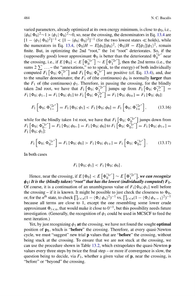
varied parameters, already optimized at its own energy minimum, is close to φ 0 , i.e.,
φ 0 | 0 2 ∼1 > φ 1 | 0 2 ∼0, so, near the crossing, the denominators in Eq. 13.4 are
[1 − −φ 1 | 0 2 ] −1 < [1 − −φ 0 | 0 2 ] −1 (for the two lowest states holds), while
the numerators in Eq. 13.4, 0 |H − E[φ 0 ]|φ 0 2 , 0 |H − E[φ 1 ]|φ 1 2 , remain
finite. But, in optimizing the 2nd “root,” the 1st “root” deteriorates. So, if the
(supposedly good) lower approximant 0 is better than the deteriorated "1r"
0
near
the crossing, i.e., if E [ 0 ] < E
"1r"
0
∼ E
“2r”
1
, then the 2nd terms (i.e., the
sums 2
. . . – the “annexations,” so to speak, to the energy) of both individually
computed F 1
0 ; “2r”
1
and F 1
0 ; "1r"
0
are positive (cf. Eq. 13.4), and, due
to the smaller denominator, the F 1 of (the continuous) φ 0 is normally larger than
the F 1 of (the continuous) φ 1 . Therefore, in passing the crossing, for the blindly
taken 2nd root, we have that F 1
0 ; “2r”
1
jumps up from F 1
0 ; “2r”
1−
=
F 1 [ 0 ; φ 1− ] = F 1 [ 0 ; φ 1 ] to F 1
0 ; “2r”
1+
= F 1 [ 0 ; φ 0+ ] = F 1 [ 0 ; φ 0 ]:
F 1
0 ;
“2r”
1−
= F 1 [ 0 ; φ 1 ] < F 1 [ 0 ; φ 0 ] = F 1
0 ;
“2r”
1+
,
(13.16)
while for the blindly taken 1st root, we have that F 1
0 ; "1r"
0
jumps down from
F 1
0 ; "1r"
0−
= F 1 [ 0 ; φ 0− ] = F 1 [ 0 ; φ 0 ] to F 1
0 ; "1r"
0+
= F 1 [ 0 ; φ 1+ ] =
F 1 [ 0 ; φ 1 ]:
F 1
0 ;
"1r"
0−
= F 1 [ 0 ; φ 0 ] > F 1 [ 0 ; φ 1+ ] = F 1
0 ;
"1r"
0+
.
(13.17)
In both cases
F 1 [ 0 ; φ 1 ] < F 1 [ 0 ; φ 0 ] .
Hence, near the crossing, if E [ 0 ] < E
"1r"
0
∼ E
“2r”
1
, we can recognize
φ 1 : It is the (blindly taken) “root” that has the lowest (individually computed) F 1 .
Of course, it is a continuation of an unambiguous value of F 1 [ 0 ; φ 1 ] well before
the crossing – if it is known. It might be possible to just check the closeness to 0 ,
or, for the n th state, to check
i < n (1 − − i | φ n 2 ) −1 vs.
i < n (1 − − i | φ n − 1 2 ) −1
because all terms are close to 1, except the one resembling some lower crude
approximant i < n , that would make it close to 0 −1 , but this possibility needs future
investigation. (Generally, the recognition of φ 1 could be used in MCSCF to feed the
next iteration.)
Yet, by just recognizing φ 1 at the crossing, we have not found the sought optimal
position of p 1 , which is “before” the crossing. Therefore, at every quasi-Newton
cycle, we must “suggest” new trial p values that are “before” the crossing, without
being stuck at the crossing. To ensure that we are not stuck at the crossing, we
can use the procedure shown in Table 13.2, which extrapolates the quasi-Newton p
values every three steps by twice the final step – or more if convergence is slow, the
question being to decide, via F 1 , whether a given value of p, near the crossing, is
“before” or “beyond” the crossing.
N. C. Bacalis
varied parameters, already optimized at its own energy minimum, is close to φ 0 , i.e.,
φ 0 | 0 2 ∼1 > φ 1 | 0 2 ∼0, so, near the crossing, the denominators in Eq. 13.4 are
[1 − −φ 1 | 0 2 ] −1 < [1 − −φ 0 | 0 2 ] −1 (for the two lowest states holds), while
the numerators in Eq. 13.4, 0 |H − E[φ 0 ]|φ 0 2 , 0 |H − E[φ 1 ]|φ 1 2 , remain
finite. But, in optimizing the 2nd “root,” the 1st “root” deteriorates. So, if the
(supposedly good) lower approximant 0 is better than the deteriorated "1r"
0
near
the crossing, i.e., if E [ 0 ] < E
"1r"
0
∼ E
“2r”
1
, then the 2nd terms (i.e., the
sums 2
. . . – the “annexations,” so to speak, to the energy) of both individually
computed F 1
0 ; “2r”
1
and F 1
0 ; "1r"
0
are positive (cf. Eq. 13.4), and, due
to the smaller denominator, the F 1 of (the continuous) φ 0 is normally larger than
the F 1 of (the continuous) φ 1 . Therefore, in passing the crossing, for the blindly
taken 2nd root, we have that F 1
0 ; “2r”
1
jumps up from F 1
0 ; “2r”
1−
=
F 1 [ 0 ; φ 1− ] = F 1 [ 0 ; φ 1 ] to F 1
0 ; “2r”
1+
= F 1 [ 0 ; φ 0+ ] = F 1 [ 0 ; φ 0 ]:
F 1
0 ;
“2r”
1−
= F 1 [ 0 ; φ 1 ] < F 1 [ 0 ; φ 0 ] = F 1
0 ;
“2r”
1+
,
(13.16)
while for the blindly taken 1st root, we have that F 1
0 ; "1r"
0
jumps down from
F 1
0 ; "1r"
0−
= F 1 [ 0 ; φ 0− ] = F 1 [ 0 ; φ 0 ] to F 1
0 ; "1r"
0+
= F 1 [ 0 ; φ 1+ ] =
F 1 [ 0 ; φ 1 ]:
F 1
0 ;
"1r"
0−
= F 1 [ 0 ; φ 0 ] > F 1 [ 0 ; φ 1+ ] = F 1
0 ;
"1r"
0+
.
(13.17)
In both cases
F 1 [ 0 ; φ 1 ] < F 1 [ 0 ; φ 0 ] .
Hence, near the crossing, if E [ 0 ] < E
"1r"
0
∼ E
“2r”
1
, we can recognize
φ 1 : It is the (blindly taken) “root” that has the lowest (individually computed) F 1 .
Of course, it is a continuation of an unambiguous value of F 1 [ 0 ; φ 1 ] well before
the crossing – if it is known. It might be possible to just check the closeness to 0 ,
or, for the n th state, to check
i < n (1 − − i | φ n 2 ) −1 vs.
i < n (1 − − i | φ n − 1 2 ) −1
because all terms are close to 1, except the one resembling some lower crude
approximant i < n , that would make it close to 0 −1 , but this possibility needs future
investigation. (Generally, the recognition of φ 1 could be used in MCSCF to feed the
next iteration.)
Yet, by just recognizing φ 1 at the crossing, we have not found the sought optimal
position of p 1 , which is “before” the crossing. Therefore, at every quasi-Newton
cycle, we must “suggest” new trial p values that are “before” the crossing, without
being stuck at the crossing. To ensure that we are not stuck at the crossing, we
can use the procedure shown in Table 13.2, which extrapolates the quasi-Newton p
values every three steps by twice the final step – or more if convergence is slow, the
question being to decide, via F 1 , whether a given value of p, near the crossing, is
“before” or “beyond” the crossing.