

13 If Truncated Wave Functions of Excited State Energy Saddle Points Are. . .
483
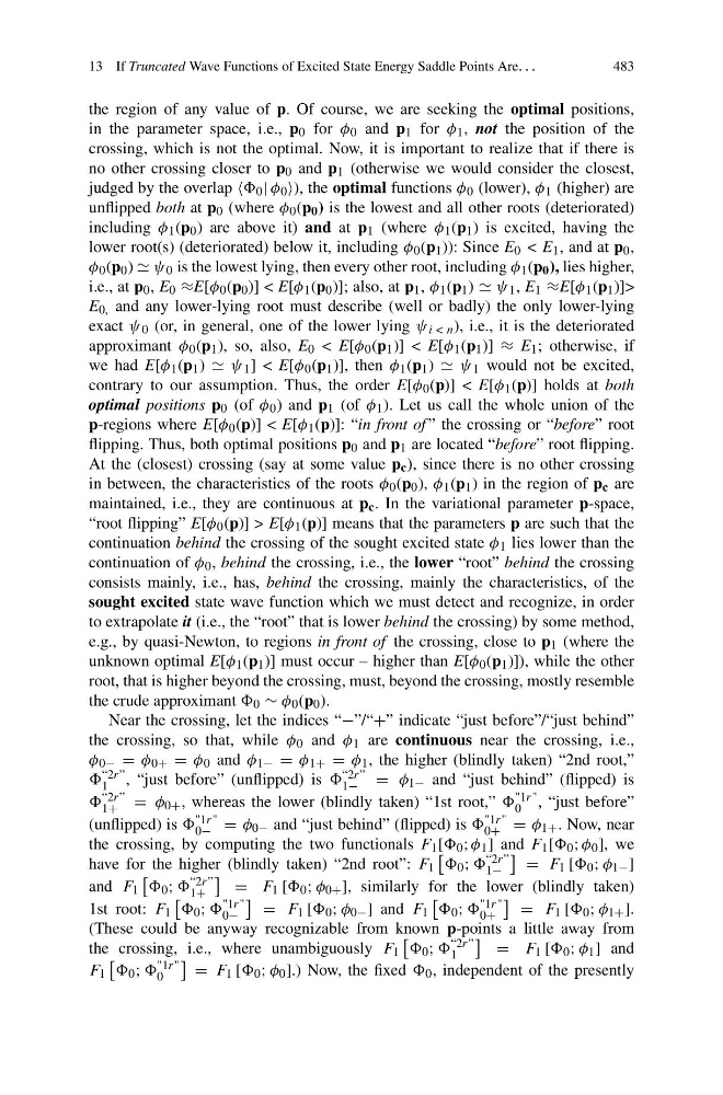
the region of any value of p. Of course, we are seeking the optimal positions,
in the parameter space, i.e., p 0 for φ 0 and p 1 for φ 1 , not the position of the
crossing, which is not the optimal. Now, it is important to realize that if there is
no other crossing closer to p 0 and p 1 (otherwise we would consider the closest,
judged by the overlap 0 | φ 0 ), the optimal functions φ 0 (lower), φ 1 (higher) are
unflipped both at p 0 (where φ 0 (p 0 ) is the lowest and all other roots (deteriorated)
including φ 1 (p 0 ) are above it) and at p 1 (where φ 1 (p 1 ) is excited, having the
lower root(s) (deteriorated) below it, including φ 0 (p 1 )): Since E 0 < E 1 , and at p 0 ,
φ 0 (p 0 ) ψ 0 is the lowest lying, then every other root, including φ 1 (p 0 ), lies higher,
i.e., at p 0 , E 0 ≈E[φ 0 (p 0 )] < E[φ 1 (p 0 )]; also, at p 1 , φ 1 (p 1 ) ψ 1 , E 1 ≈E[φ 1 (p 1 )]>
E 0, and any lower-lying root must describe (well or badly) the only lower-lying
exact ψ 0 (or, in general, one of the lower lying ψ i < n ), i.e., it is the deteriorated
approximant φ 0 (p 1 ), so, also, E 0 < E[φ 0 (p 1 )] < E[φ 1 (p 1 )] ≈ E 1 ; otherwise, if
we had E[φ 1 (p 1 ) ψ 1 ] < E[φ 0 (p 1 )], then φ 1 (p 1 ) ψ 1 would not be excited,
contrary to our assumption. Thus, the order E[φ 0 (p)] < E[φ 1 (p)] holds at both
optimal positions p 0 (of φ 0 ) and p 1 (of φ 1 ). Let us call the whole union of the
p-regions where E[φ 0 (p)] < E[φ 1 (p)]: “in front of ” the crossing or “before” root
flipping. Thus, both optimal positions p 0 and p 1 are located “before” root flipping.
At the (closest) crossing (say at some value p c ), since there is no other crossing
in between, the characteristics of the roots φ 0 (p 0 ), φ 1 (p 1 ) in the region of p c are
maintained, i.e., they are continuous at p c . In the variational parameter p-space,
“root flipping” E[φ 0 (p)] > E[φ 1 (p)] means that the parameters p are such that the
continuation behind the crossing of the sought excited state φ 1 lies lower than the
continuation of φ 0 , behind the crossing, i.e., the lower “root” behind the crossing
consists mainly, i.e., has, behind the crossing, mainly the characteristics, of the
sought excited state wave function which we must detect and recognize, in order
to extrapolate it (i.e., the “root” that is lower behind the crossing) by some method,
e.g., by quasi-Newton, to regions in front of the crossing, close to p 1 (where the
unknown optimal E[φ 1 (p 1 )] must occur – higher than E[φ 0 (p 1 )]), while the other
root, that is higher beyond the crossing, must, beyond the crossing, mostly resemble
the crude approximant 0 ∼ φ 0 (p 0 ).
Near the crossing, let the indices “−”/“+” indicate “just before”/“just behind”
the crossing, so that, while φ 0 and φ 1 are continuous near the crossing, i.e.,
φ 0− = φ 0+ = φ 0 and φ 1− = φ 1+ = φ 1 , the higher (blindly taken) “2nd root,”
“2r”
1 , “just before” (unflipped) is “2r”
1− = φ 1− and “just behind” (flipped) is
“2r”
1+ = φ 0+ , whereas the lower (blindly taken) “1st root,” "1r"
0 , “just before”
(unflipped) is "1r"
0− = φ 0− and “just behind” (flipped) is "1r"
0+ = φ 1+ . Now, near
the crossing, by computing the two functionals F 1 [ 0 ; φ 1 ] and F 1 [ 0 ; φ 0 ], we
have for the higher (blindly taken) “2nd root”: F 1
0 ; “2r”
1−
= F 1 [ 0 ; φ 1− ]
and F 1
0 ; “2r”
1+
= F 1 [ 0 ; φ 0+ ], similarly for the lower (blindly taken)
1st root: F 1
0 ; "1r"
0−
= F 1 [ 0 ; φ 0− ] and F 1
0 ; "1r"
0+
= F 1 [ 0 ; φ 1+ ].
(These could be anyway recognizable from known p-points a little away from
the crossing, i.e., where unambiguously F 1
0 ; “2r”
1
= F 1 [ 0 ; φ 1 ] and
F 1
0 ; "1r"
0
= F 1 [ 0 ; φ 0 ].) Now, the fixed 0 , independent of the presently
483
the region of any value of p. Of course, we are seeking the optimal positions,
in the parameter space, i.e., p 0 for φ 0 and p 1 for φ 1 , not the position of the
crossing, which is not the optimal. Now, it is important to realize that if there is
no other crossing closer to p 0 and p 1 (otherwise we would consider the closest,
judged by the overlap 0 | φ 0 ), the optimal functions φ 0 (lower), φ 1 (higher) are
unflipped both at p 0 (where φ 0 (p 0 ) is the lowest and all other roots (deteriorated)
including φ 1 (p 0 ) are above it) and at p 1 (where φ 1 (p 1 ) is excited, having the
lower root(s) (deteriorated) below it, including φ 0 (p 1 )): Since E 0 < E 1 , and at p 0 ,
φ 0 (p 0 ) ψ 0 is the lowest lying, then every other root, including φ 1 (p 0 ), lies higher,
i.e., at p 0 , E 0 ≈E[φ 0 (p 0 )] < E[φ 1 (p 0 )]; also, at p 1 , φ 1 (p 1 ) ψ 1 , E 1 ≈E[φ 1 (p 1 )]>
E 0, and any lower-lying root must describe (well or badly) the only lower-lying
exact ψ 0 (or, in general, one of the lower lying ψ i < n ), i.e., it is the deteriorated
approximant φ 0 (p 1 ), so, also, E 0 < E[φ 0 (p 1 )] < E[φ 1 (p 1 )] ≈ E 1 ; otherwise, if
we had E[φ 1 (p 1 ) ψ 1 ] < E[φ 0 (p 1 )], then φ 1 (p 1 ) ψ 1 would not be excited,
contrary to our assumption. Thus, the order E[φ 0 (p)] < E[φ 1 (p)] holds at both
optimal positions p 0 (of φ 0 ) and p 1 (of φ 1 ). Let us call the whole union of the
p-regions where E[φ 0 (p)] < E[φ 1 (p)]: “in front of ” the crossing or “before” root
flipping. Thus, both optimal positions p 0 and p 1 are located “before” root flipping.
At the (closest) crossing (say at some value p c ), since there is no other crossing
in between, the characteristics of the roots φ 0 (p 0 ), φ 1 (p 1 ) in the region of p c are
maintained, i.e., they are continuous at p c . In the variational parameter p-space,
“root flipping” E[φ 0 (p)] > E[φ 1 (p)] means that the parameters p are such that the
continuation behind the crossing of the sought excited state φ 1 lies lower than the
continuation of φ 0 , behind the crossing, i.e., the lower “root” behind the crossing
consists mainly, i.e., has, behind the crossing, mainly the characteristics, of the
sought excited state wave function which we must detect and recognize, in order
to extrapolate it (i.e., the “root” that is lower behind the crossing) by some method,
e.g., by quasi-Newton, to regions in front of the crossing, close to p 1 (where the
unknown optimal E[φ 1 (p 1 )] must occur – higher than E[φ 0 (p 1 )]), while the other
root, that is higher beyond the crossing, must, beyond the crossing, mostly resemble
the crude approximant 0 ∼ φ 0 (p 0 ).
Near the crossing, let the indices “−”/“+” indicate “just before”/“just behind”
the crossing, so that, while φ 0 and φ 1 are continuous near the crossing, i.e.,
φ 0− = φ 0+ = φ 0 and φ 1− = φ 1+ = φ 1 , the higher (blindly taken) “2nd root,”
“2r”
1 , “just before” (unflipped) is “2r”
1− = φ 1− and “just behind” (flipped) is
“2r”
1+ = φ 0+ , whereas the lower (blindly taken) “1st root,” "1r"
0 , “just before”
(unflipped) is "1r"
0− = φ 0− and “just behind” (flipped) is "1r"
0+ = φ 1+ . Now, near
the crossing, by computing the two functionals F 1 [ 0 ; φ 1 ] and F 1 [ 0 ; φ 0 ], we
have for the higher (blindly taken) “2nd root”: F 1
0 ; “2r”
1−
= F 1 [ 0 ; φ 1− ]
and F 1
0 ; “2r”
1+
= F 1 [ 0 ; φ 0+ ], similarly for the lower (blindly taken)
1st root: F 1
0 ; "1r"
0−
= F 1 [ 0 ; φ 0− ] and F 1
0 ; "1r"
0+
= F 1 [ 0 ; φ 1+ ].
(These could be anyway recognizable from known p-points a little away from
the crossing, i.e., where unambiguously F 1
0 ; “2r”
1
= F 1 [ 0 ; φ 1 ] and
F 1
0 ; "1r"
0
= F 1 [ 0 ; φ 0 ].) Now, the fixed 0 , independent of the presently