

5 Enabling Materials By Dimensionality: From 0D to 3D Carbon-Based. . .
177
where the G = G = 0 limit results in an average over the unit cell of the
corresponding microscopic quantity, which can exhibit rapid oscillations at the
atomic level.
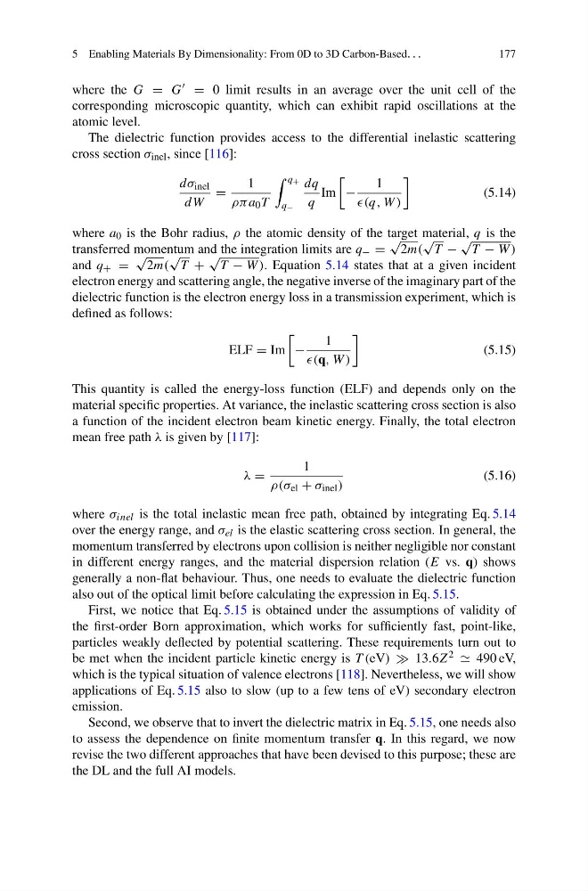
The dielectric function provides access to the differential inelastic scattering
cross section σ inel , since [116]:
dσ inel
dW
=
1
ρπa 0 T
q +
q −
dq
q
Im
−
1
(q, W )
(5.14)
where a 0 is the Bohr radius, ρ the atomic density of the target material, q is the
transferred momentum and the integration limits are q − =
√
2m(
√
T −
√
T − W )
and q + =
√
2m(
√
T +
√
T − W ). Equation 5.14 states that at a given incident
electron energy and scattering angle, the negative inverse of the imaginary part of the
dielectric function is the electron energy loss in a transmission experiment, which is
defined as follows:
ELF = Im
−
1
(q, W )
(5.15)
This quantity is called the energy-loss function (ELF) and depends only on the
material specific properties. At variance, the inelastic scattering cross section is also
a function of the incident electron beam kinetic energy. Finally, the total electron
mean free path λ is given by [117]:
λ =
1
ρ(σ el + σ inel )
(5.16)
where σ inel is the total inelastic mean free path, obtained by integrating Eq. 5.14
over the energy range, and σ el is the elastic scattering cross section. In general, the
momentum transferred by electrons upon collision is neither negligible nor constant
in different energy ranges, and the material dispersion relation (E vs. q) shows
generally a non-flat behaviour. Thus, one needs to evaluate the dielectric function
also out of the optical limit before calculating the expression in Eq. 5.15.
First, we notice that Eq. 5.15 is obtained under the assumptions of validity of
the first-order Born approximation, which works for sufficiently fast, point-like,
particles weakly deflected by potential scattering. These requirements turn out to
be met when the incident particle kinetic energy is T (eV) 13.6Z 2 490 eV,
which is the typical situation of valence electrons [118]. Nevertheless, we will show
applications of Eq. 5.15 also to slow (up to a few tens of eV) secondary electron
emission.
Second, we observe that to invert the dielectric matrix in Eq. 5.15, one needs also
to assess the dependence on finite momentum transfer q. In this regard, we now
revise the two different approaches that have been devised to this purpose; these are
the DL and the full AI models.
177
where the G = G = 0 limit results in an average over the unit cell of the
corresponding microscopic quantity, which can exhibit rapid oscillations at the
atomic level.
The dielectric function provides access to the differential inelastic scattering
cross section σ inel , since [116]:
dσ inel
dW
=
1
ρπa 0 T
q +
q −
dq
q
Im
−
1
(q, W )
(5.14)
where a 0 is the Bohr radius, ρ the atomic density of the target material, q is the
transferred momentum and the integration limits are q − =
√
2m(
√
T −
√
T − W )
and q + =
√
2m(
√
T +
√
T − W ). Equation 5.14 states that at a given incident
electron energy and scattering angle, the negative inverse of the imaginary part of the
dielectric function is the electron energy loss in a transmission experiment, which is
defined as follows:
ELF = Im
−
1
(q, W )
(5.15)
This quantity is called the energy-loss function (ELF) and depends only on the
material specific properties. At variance, the inelastic scattering cross section is also
a function of the incident electron beam kinetic energy. Finally, the total electron
mean free path λ is given by [117]:
λ =
1
ρ(σ el + σ inel )
(5.16)
where σ inel is the total inelastic mean free path, obtained by integrating Eq. 5.14
over the energy range, and σ el is the elastic scattering cross section. In general, the
momentum transferred by electrons upon collision is neither negligible nor constant
in different energy ranges, and the material dispersion relation (E vs. q) shows
generally a non-flat behaviour. Thus, one needs to evaluate the dielectric function
also out of the optical limit before calculating the expression in Eq. 5.15.
First, we notice that Eq. 5.15 is obtained under the assumptions of validity of
the first-order Born approximation, which works for sufficiently fast, point-like,
particles weakly deflected by potential scattering. These requirements turn out to
be met when the incident particle kinetic energy is T (eV) 13.6Z 2 490 eV,
which is the typical situation of valence electrons [118]. Nevertheless, we will show
applications of Eq. 5.15 also to slow (up to a few tens of eV) secondary electron
emission.
Second, we observe that to invert the dielectric matrix in Eq. 5.15, one needs also
to assess the dependence on finite momentum transfer q. In this regard, we now
revise the two different approaches that have been devised to this purpose; these are
the DL and the full AI models.