

100
S. Yanagisawa and I. Hamada
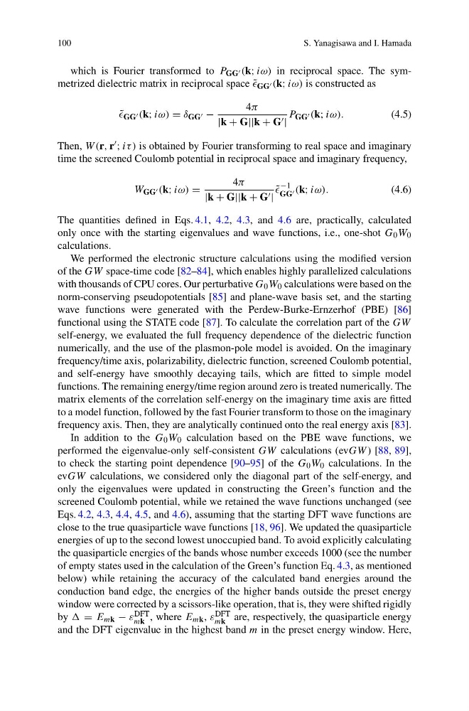
which is Fourier transformed to P GG (k; iω) in reciprocal space. The symmetrized dielectric matrix in reciprocal space ˜
GG (k; iω) is constructed as
˜
GG (k; iω) = δ GG −
4π
|k + G||k + G |
P GG (k; iω).
(4.5)
Then, W (r, r ; iτ ) is obtained by Fourier transforming to real space and imaginary
time the screened Coulomb potential in reciprocal space and imaginary frequency,
W GG (k; iω) =
4π
|k + G||k + G |
˜
−1
GG (k; iω).
(4.6)
The quantities defined in Eqs. 4.1, 4.2, 4.3, and 4.6 are, practically, calculated
only once with the starting eigenvalues and wave functions, i.e., one-shot G 0 W 0
calculations.
We performed the electronic structure calculations using the modified version
of the GW space-time code [82–84], which enables highly parallelized calculations
with thousands of CPU cores. Our perturbative G 0 W 0 calculations were based on the
norm-conserving pseudopotentials [85] and plane-wave basis set, and the starting
wave functions were generated with the Perdew-Burke-Ernzerhof (PBE) [86]
functional using the STATE code [87]. To calculate the correlation part of the GW
self-energy, we evaluated the full frequency dependence of the dielectric function
numerically, and the use of the plasmon-pole model is avoided. On the imaginary
frequency/time axis, polarizability, dielectric function, screened Coulomb potential,
and self-energy have smoothly decaying tails, which are fitted to simple model
functions. The remaining energy/time region around zero is treated numerically. The
matrix elements of the correlation self-energy on the imaginary time axis are fitted
to a model function, followed by the fast Fourier transform to those on the imaginary
frequency axis. Then, they are analytically continued onto the real energy axis [83].
In addition to the G 0 W 0 calculation based on the PBE wave functions, we
performed the eigenvalue-only self-consistent GW calculations (evGW ) [88, 89],
to check the starting point dependence [90–95] of the G 0 W 0 calculations. In the
evGW calculations, we considered only the diagonal part of the self-energy, and
only the eigenvalues were updated in constructing the Green’s function and the
screened Coulomb potential, while we retained the wave functions unchanged (see
Eqs. 4.2, 4.3, 4.4, 4.5, and 4.6), assuming that the starting DFT wave functions are
close to the true quasiparticle wave functions [18, 96]. We updated the quasiparticle
energies of up to the second lowest unoccupied band. To avoid explicitly calculating
the quasiparticle energies of the bands whose number exceeds 1000 (see the number
of empty states used in the calculation of the Green’s function Eq. 4.3, as mentioned
below) while retaining the accuracy of the calculated band energies around the
conduction band edge, the energies of the higher bands outside the preset energy
window were corrected by a scissors-like operation, that is, they were shifted rigidly
by = E mk − ε DFT
mk , where E mk , ε DFT
mk are, respectively, the quasiparticle energy
and the DFT eigenvalue in the highest band m in the preset energy window. Here,
S. Yanagisawa and I. Hamada
which is Fourier transformed to P GG (k; iω) in reciprocal space. The symmetrized dielectric matrix in reciprocal space ˜
GG (k; iω) is constructed as
˜
GG (k; iω) = δ GG −
4π
|k + G||k + G |
P GG (k; iω).
(4.5)
Then, W (r, r ; iτ ) is obtained by Fourier transforming to real space and imaginary
time the screened Coulomb potential in reciprocal space and imaginary frequency,
W GG (k; iω) =
4π
|k + G||k + G |
˜
−1
GG (k; iω).
(4.6)
The quantities defined in Eqs. 4.1, 4.2, 4.3, and 4.6 are, practically, calculated
only once with the starting eigenvalues and wave functions, i.e., one-shot G 0 W 0
calculations.
We performed the electronic structure calculations using the modified version
of the GW space-time code [82–84], which enables highly parallelized calculations
with thousands of CPU cores. Our perturbative G 0 W 0 calculations were based on the
norm-conserving pseudopotentials [85] and plane-wave basis set, and the starting
wave functions were generated with the Perdew-Burke-Ernzerhof (PBE) [86]
functional using the STATE code [87]. To calculate the correlation part of the GW
self-energy, we evaluated the full frequency dependence of the dielectric function
numerically, and the use of the plasmon-pole model is avoided. On the imaginary
frequency/time axis, polarizability, dielectric function, screened Coulomb potential,
and self-energy have smoothly decaying tails, which are fitted to simple model
functions. The remaining energy/time region around zero is treated numerically. The
matrix elements of the correlation self-energy on the imaginary time axis are fitted
to a model function, followed by the fast Fourier transform to those on the imaginary
frequency axis. Then, they are analytically continued onto the real energy axis [83].
In addition to the G 0 W 0 calculation based on the PBE wave functions, we
performed the eigenvalue-only self-consistent GW calculations (evGW ) [88, 89],
to check the starting point dependence [90–95] of the G 0 W 0 calculations. In the
evGW calculations, we considered only the diagonal part of the self-energy, and
only the eigenvalues were updated in constructing the Green’s function and the
screened Coulomb potential, while we retained the wave functions unchanged (see
Eqs. 4.2, 4.3, 4.4, 4.5, and 4.6), assuming that the starting DFT wave functions are
close to the true quasiparticle wave functions [18, 96]. We updated the quasiparticle
energies of up to the second lowest unoccupied band. To avoid explicitly calculating
the quasiparticle energies of the bands whose number exceeds 1000 (see the number
of empty states used in the calculation of the Green’s function Eq. 4.3, as mentioned
below) while retaining the accuracy of the calculated band energies around the
conduction band edge, the energies of the higher bands outside the preset energy
window were corrected by a scissors-like operation, that is, they were shifted rigidly
by = E mk − ε DFT
mk , where E mk , ε DFT
mk are, respectively, the quasiparticle energy
and the DFT eigenvalue in the highest band m in the preset energy window. Here,