

Processes 2019, 7,20
√
ε = 0.25 ≫ 0.1141 and thus, s max = 4 is not satisfied. Moreover, for a setting like τ d = 40 ms and
C m = 2
μF
m 2 one diverges more from the condition
√
ε ≪ 0.1141, since
√
ε = 1/
√ 2. However, the system
still exhibits MMOs or EADs but does not satisfy (12), since the condition
√
ε ≪ μ is barely to fulfil.
Our next step is the study of system (1) using bifurcation analysis. In general, a bifurcation of a
dynamical system is a qualitative change in its dynamics produced by varying parameters. Since we
investigate the occurrence of EADs induced by an enhancement in the calcium current I Ca 2+ , we will
choose the conductance G Ca 2+ as bifurcation parameter to be able to simulate the decreasing or mainly
the increasing of the calcium current. Moreover, we will use our observation from above to analyse the
behaviour of system (1). First of all, determining the equilibrium curve of system (1), which is basically
the equilibria of this system for different values of G Ca 2+ , yields two stable branches and one unstable
branch for all parameter settings. Depending on the parameter setting the equilibrium curve loses or
wins stability via a sub- or supercritical Andronov-Hopf bifurcation, cf. also [15]. An Andronov-Hopf
bifurcation is characterised by a pair of purely imaginary eigenvalues, where the equilibrium changes
stability and a unique limit cycle bifurcates from it, i.e., it is the birth of a limit cycle. The distinction
into sub- or supercritical means that an unstable or stable limit cycle, respectively, bifurcates. For the
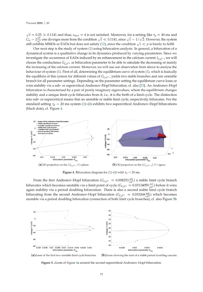
standard setting τ d = 20 ms system (1)–(4) exhibits two supercritical Andronov-Hopf bifurcations
(black dots), cf. Figure 4.
0.01
0.015
0.02
0.025
0.03
bifurcation parameter G Ca
-80
-60
-40
-20
0
20
voltage V (mV)
supercritical Andronov-Hopf bifurcation
stable equilibrium branch
unstable equilibrium branch
stable limit cycle branch
unstable limit cycle branch
period doubling bifurcation
limit point of cycles
(a) 2D projection on the (G Ca 2+ , V)–plane.
(b) 3D projection on the (G Ca 2+ , f , V)–space.
Figure 4. Bifurcation diagram for (1)–(4) with τ d = 20 ms.
From the first Andronov-Hopf bifurcation (G Ca 2+ ≈ 0.008253
mS
cm 2 ) a stable limit cycle branch
bifurcates which becomes unstable via a limit point of cycle (G Ca 2+ ≈ 0.03134055
mS
cm 2 ) before it wins
again stability via a period doubling bifurcation. There is also a second stable limit cycle branch
bifurcating from the second Andronov-Hopf bifurcation (G Ca 2+ ≈ 0.033268
mS
cm 2 ) which becomes
unstable via a period doubling bifurcation (connection of both limit cycle branches), cf. also Figure 5b.
0.029 0.0295 0.03 0.0305 0.031 0.0315 0.032 0.0325 0.033
bifurcation parameter G Ca
-80
-60
-40
-20
0
20
voltage V (mV)
(a)Zoom of the first two unstable limit cycle branches.
0.0329
0.033
0.0331
0.0332
bifurcation parameter G Ca
-36
-34
-32
-30
-28
-26
-24
-22
-20
voltage V (mV)
(b)Zoom showing the start of a stable period doubling cascade.
Figure 5. Zoom of Figure 4a around the second supercritical Andronov-Hopf bifurcation.
73
√
ε = 0.25 ≫ 0.1141 and thus, s max = 4 is not satisfied. Moreover, for a setting like τ d = 40 ms and
C m = 2
μF
m 2 one diverges more from the condition
√
ε ≪ 0.1141, since
√
ε = 1/
√ 2. However, the system
still exhibits MMOs or EADs but does not satisfy (12), since the condition
√
ε ≪ μ is barely to fulfil.
Our next step is the study of system (1) using bifurcation analysis. In general, a bifurcation of a
dynamical system is a qualitative change in its dynamics produced by varying parameters. Since we
investigate the occurrence of EADs induced by an enhancement in the calcium current I Ca 2+ , we will
choose the conductance G Ca 2+ as bifurcation parameter to be able to simulate the decreasing or mainly
the increasing of the calcium current. Moreover, we will use our observation from above to analyse the
behaviour of system (1). First of all, determining the equilibrium curve of system (1), which is basically
the equilibria of this system for different values of G Ca 2+ , yields two stable branches and one unstable
branch for all parameter settings. Depending on the parameter setting the equilibrium curve loses or
wins stability via a sub- or supercritical Andronov-Hopf bifurcation, cf. also [15]. An Andronov-Hopf
bifurcation is characterised by a pair of purely imaginary eigenvalues, where the equilibrium changes
stability and a unique limit cycle bifurcates from it, i.e., it is the birth of a limit cycle. The distinction
into sub- or supercritical means that an unstable or stable limit cycle, respectively, bifurcates. For the
standard setting τ d = 20 ms system (1)–(4) exhibits two supercritical Andronov-Hopf bifurcations
(black dots), cf. Figure 4.
0.01
0.015
0.02
0.025
0.03
bifurcation parameter G Ca
-80
-60
-40
-20
0
20
voltage V (mV)
supercritical Andronov-Hopf bifurcation
stable equilibrium branch
unstable equilibrium branch
stable limit cycle branch
unstable limit cycle branch
period doubling bifurcation
limit point of cycles
(a) 2D projection on the (G Ca 2+ , V)–plane.
(b) 3D projection on the (G Ca 2+ , f , V)–space.
Figure 4. Bifurcation diagram for (1)–(4) with τ d = 20 ms.
From the first Andronov-Hopf bifurcation (G Ca 2+ ≈ 0.008253
mS
cm 2 ) a stable limit cycle branch
bifurcates which becomes unstable via a limit point of cycle (G Ca 2+ ≈ 0.03134055
mS
cm 2 ) before it wins
again stability via a period doubling bifurcation. There is also a second stable limit cycle branch
bifurcating from the second Andronov-Hopf bifurcation (G Ca 2+ ≈ 0.033268
mS
cm 2 ) which becomes
unstable via a period doubling bifurcation (connection of both limit cycle branches), cf. also Figure 5b.
0.029 0.0295 0.03 0.0305 0.031 0.0315 0.032 0.0325 0.033
bifurcation parameter G Ca
-80
-60
-40
-20
0
20
voltage V (mV)
(a)Zoom of the first two unstable limit cycle branches.
0.0329
0.033
0.0331
0.0332
bifurcation parameter G Ca
-36
-34
-32
-30
-28
-26
-24
-22
-20
voltage V (mV)
(b)Zoom showing the start of a stable period doubling cascade.
Figure 5. Zoom of Figure 4a around the second supercritical Andronov-Hopf bifurcation.
73