

Processes 2019, 7,20
This unstable limit cycle branch has of course influence on the system (1) but it does not
yields automatically EADs, it also may correspond to an AP. Notice that the limit cycle branches
are determined via a continuation algorithm included in MATCONT. The region between the first
Andronov-Hopf bifurcation and the first limit point of cycle (G Ca 2+ ≈ 0.03134055
mS
cm 2 ) indicates the
region, where no EADs occur, cf. [15]. EADs appear after the first limit point of cycle. In Figure 5a the
transient from AP to EADs via the limit point of cycle bifurcation is highlighted, while Figure 5b shows
the beginning of a stable period doubling cascade. In Figure 9 we see that this transient might be also
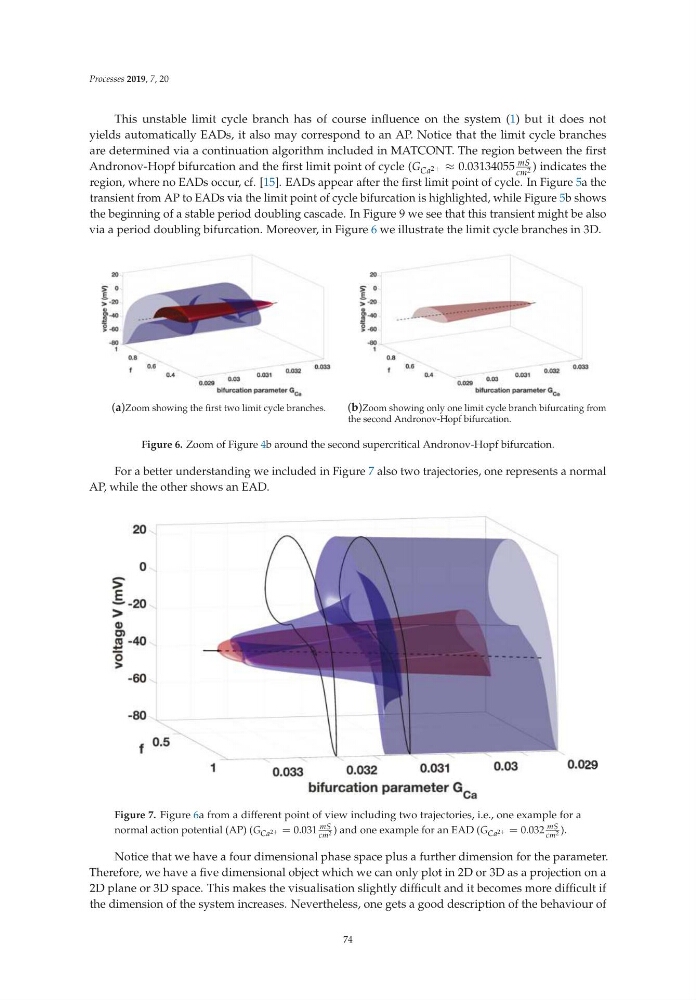
via a period doubling bifurcation. Moreover, in Figure 6 we illustrate the limit cycle branches in 3D.
(a)Zoom showing the first two limit cycle branches.
(b)Zoom showing only one limit cycle branch bifurcating from
the second Andronov-Hopf bifurcation.
Figure 6. Zoom of Figure 4b around the second supercritical Andronov-Hopf bifurcation.
For a better understanding we included in Figure 7 also two trajectories, one represents a normal
AP, while the other shows an EAD.
Figure 7. Figure 6a from a different point of view including two trajectories, i.e., one example for a
normal action potential (AP) (G Ca 2+ = 0.031
mS
cm 2 ) and one example for an EAD (G Ca 2+ = 0.032
mS
cm 2 ).
Notice that we have a four dimensional phase space plus a further dimension for the parameter.
Therefore, we have a five dimensional object which we can only plot in 2D or 3D as a projection on a
2D plane or 3D space. This makes the visualisation slightly difficult and it becomes more difficult if
the dimension of the system increases. Nevertheless, one gets a good description of the behaviour of
74
This unstable limit cycle branch has of course influence on the system (1) but it does not
yields automatically EADs, it also may correspond to an AP. Notice that the limit cycle branches
are determined via a continuation algorithm included in MATCONT. The region between the first
Andronov-Hopf bifurcation and the first limit point of cycle (G Ca 2+ ≈ 0.03134055
mS
cm 2 ) indicates the
region, where no EADs occur, cf. [15]. EADs appear after the first limit point of cycle. In Figure 5a the
transient from AP to EADs via the limit point of cycle bifurcation is highlighted, while Figure 5b shows
the beginning of a stable period doubling cascade. In Figure 9 we see that this transient might be also
via a period doubling bifurcation. Moreover, in Figure 6 we illustrate the limit cycle branches in 3D.
(a)Zoom showing the first two limit cycle branches.
(b)Zoom showing only one limit cycle branch bifurcating from
the second Andronov-Hopf bifurcation.
Figure 6. Zoom of Figure 4b around the second supercritical Andronov-Hopf bifurcation.
For a better understanding we included in Figure 7 also two trajectories, one represents a normal
AP, while the other shows an EAD.
Figure 7. Figure 6a from a different point of view including two trajectories, i.e., one example for a
normal action potential (AP) (G Ca 2+ = 0.031
mS
cm 2 ) and one example for an EAD (G Ca 2+ = 0.032
mS
cm 2 ).
Notice that we have a four dimensional phase space plus a further dimension for the parameter.
Therefore, we have a five dimensional object which we can only plot in 2D or 3D as a projection on a
2D plane or 3D space. This makes the visualisation slightly difficult and it becomes more difficult if
the dimension of the system increases. Nevertheless, one gets a good description of the behaviour of
74