

Processes 2019, 7,20
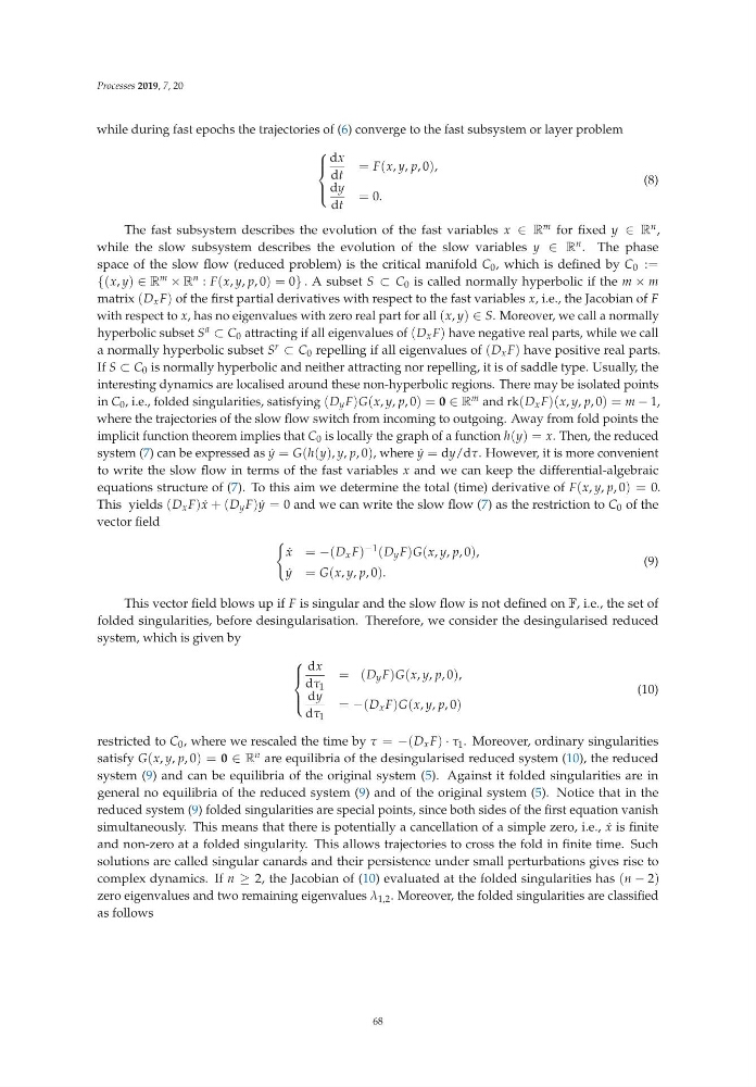
while during fast epochs the trajectories of (6) converge to the fast subsystem or layer problem
⎧
⎪
⎨
⎪
⎩
dx
dt
= F(x, y, p,0),
dy
dt
= 0.
(8)
The fast subsystem describes the evolution of the fast variables x ∈ R m for fixed y ∈ R n ,
while the slow subsystem describes the evolution of the slow variables y ∈ R n . The phase
space of the slow flow (reduced problem) is the critical manifold C 0 , which is defined by C 0 :=
{(x, y) ∈ R m × R n : F(x, y, p,0)=0} . A subset S ⊂ C 0 is called normally hyperbolic if the m × m
matrix (D x F) of the first partial derivatives with respect to the fast variables x, i.e., the Jacobian of F
with respect to x, has no eigenvalues with zero real part for all (x, y) ∈ S. Moreover, we call a normally
hyperbolic subset S a ⊂ C 0 attracting if all eigenvalues of (D x F) have negative real parts, while we call
a normally hyperbolic subset S r ⊂ C 0 repelling if all eigenvalues of (D x F) have positive real parts.
If S ⊂ C 0 is normally hyperbolic and neither attracting nor repelling, it is of saddle type. Usually, the
interesting dynamics are localised around these non-hyperbolic regions. There may be isolated points
in C 0 , i.e., folded singularities, satisfying (D y F)G(x, y, p,0)=0 ∈ R m and rk(D x F)(x, y, p,0)=m − 1,
where the trajectories of the slow flow switch from incoming to outgoing. Away from fold points the
implicit function theorem implies that C 0 is locally the graph of a function h(y)=x. Then, the reduced
system (7) can be expressed as ˙
y = G(h(y), y, p,0), where ˙
y = dy/dτ. However, it is more convenient
to write the slow flow in terms of the fast variables x and we can keep the differential-algebraic
equations structure of (7). To this aim we determine the total (time) derivative of F(x, y, p,0)=0.
This yields (D x F) ˙
x +(D y F) ˙
y = 0 and we can write the slow flow (7) as the restriction to C 0 of the
vector field
˙
x = −(D x F) −1 (D y F)G(x, y, p,0),
˙
y = G(x, y, p,0).
(9)
This vector field blows up if F is singular and the slow flow is not defined on F, i.e., the set of
folded singularities, before desingularisation. Therefore, we consider the desingularised reduced
system, which is given by
⎧
⎪
⎨
⎪
⎩
dx
dτ 1
=( D y F)G(x, y, p,0),
dy
dτ 1
= −(D x F)G(x, y, p,0)
(10)
restricted to C 0 , where we rescaled the time by τ = −(D x F) · τ 1 . Moreover, ordinary singularities
satisfy G(x, y, p,0)=0 ∈ R n are equilibria of the desingularised reduced system (10), the reduced
system (9) and can be equilibria of the original system (5). Against it folded singularities are in
general no equilibria of the reduced system (9) and of the original system (5). Notice that in the
reduced system (9) folded singularities are special points, since both sides of the first equation vanish
simultaneously. This means that there is potentially a cancellation of a simple zero, i.e., ˙
x is finite
and non-zero at a folded singularity. This allows trajectories to cross the fold in finite time. Such
solutions are called singular canards and their persistence under small perturbations gives rise to
complex dynamics. If n ≥ 2, the Jacobian of (10) evaluated at the folded singularities has (n − 2)
zero eigenvalues and two remaining eigenvalues λ 1,2 . Moreover, the folded singularities are classified
as follows
68
while during fast epochs the trajectories of (6) converge to the fast subsystem or layer problem
⎧
⎪
⎨
⎪
⎩
dx
dt
= F(x, y, p,0),
dy
dt
= 0.
(8)
The fast subsystem describes the evolution of the fast variables x ∈ R m for fixed y ∈ R n ,
while the slow subsystem describes the evolution of the slow variables y ∈ R n . The phase
space of the slow flow (reduced problem) is the critical manifold C 0 , which is defined by C 0 :=
{(x, y) ∈ R m × R n : F(x, y, p,0)=0} . A subset S ⊂ C 0 is called normally hyperbolic if the m × m
matrix (D x F) of the first partial derivatives with respect to the fast variables x, i.e., the Jacobian of F
with respect to x, has no eigenvalues with zero real part for all (x, y) ∈ S. Moreover, we call a normally
hyperbolic subset S a ⊂ C 0 attracting if all eigenvalues of (D x F) have negative real parts, while we call
a normally hyperbolic subset S r ⊂ C 0 repelling if all eigenvalues of (D x F) have positive real parts.
If S ⊂ C 0 is normally hyperbolic and neither attracting nor repelling, it is of saddle type. Usually, the
interesting dynamics are localised around these non-hyperbolic regions. There may be isolated points
in C 0 , i.e., folded singularities, satisfying (D y F)G(x, y, p,0)=0 ∈ R m and rk(D x F)(x, y, p,0)=m − 1,
where the trajectories of the slow flow switch from incoming to outgoing. Away from fold points the
implicit function theorem implies that C 0 is locally the graph of a function h(y)=x. Then, the reduced
system (7) can be expressed as ˙
y = G(h(y), y, p,0), where ˙
y = dy/dτ. However, it is more convenient
to write the slow flow in terms of the fast variables x and we can keep the differential-algebraic
equations structure of (7). To this aim we determine the total (time) derivative of F(x, y, p,0)=0.
This yields (D x F) ˙
x +(D y F) ˙
y = 0 and we can write the slow flow (7) as the restriction to C 0 of the
vector field
˙
x = −(D x F) −1 (D y F)G(x, y, p,0),
˙
y = G(x, y, p,0).
(9)
This vector field blows up if F is singular and the slow flow is not defined on F, i.e., the set of
folded singularities, before desingularisation. Therefore, we consider the desingularised reduced
system, which is given by
⎧
⎪
⎨
⎪
⎩
dx
dτ 1
=( D y F)G(x, y, p,0),
dy
dτ 1
= −(D x F)G(x, y, p,0)
(10)
restricted to C 0 , where we rescaled the time by τ = −(D x F) · τ 1 . Moreover, ordinary singularities
satisfy G(x, y, p,0)=0 ∈ R n are equilibria of the desingularised reduced system (10), the reduced
system (9) and can be equilibria of the original system (5). Against it folded singularities are in
general no equilibria of the reduced system (9) and of the original system (5). Notice that in the
reduced system (9) folded singularities are special points, since both sides of the first equation vanish
simultaneously. This means that there is potentially a cancellation of a simple zero, i.e., ˙
x is finite
and non-zero at a folded singularity. This allows trajectories to cross the fold in finite time. Such
solutions are called singular canards and their persistence under small perturbations gives rise to
complex dynamics. If n ≥ 2, the Jacobian of (10) evaluated at the folded singularities has (n − 2)
zero eigenvalues and two remaining eigenvalues λ 1,2 . Moreover, the folded singularities are classified
as follows
68