

Processes 2019, 7,20
very similar to the three dimensional system, provided τ d is small enough and the other system
parameters are the same. Moreover, we want to highlight that in [1] the authors basically studied the
influence of τ x → ∞, while in [15] the influence of mainly G Ca 2+ and G K + is investigated. In this paper,
we are focused on the influence of more system parameter and the identification of their importance.
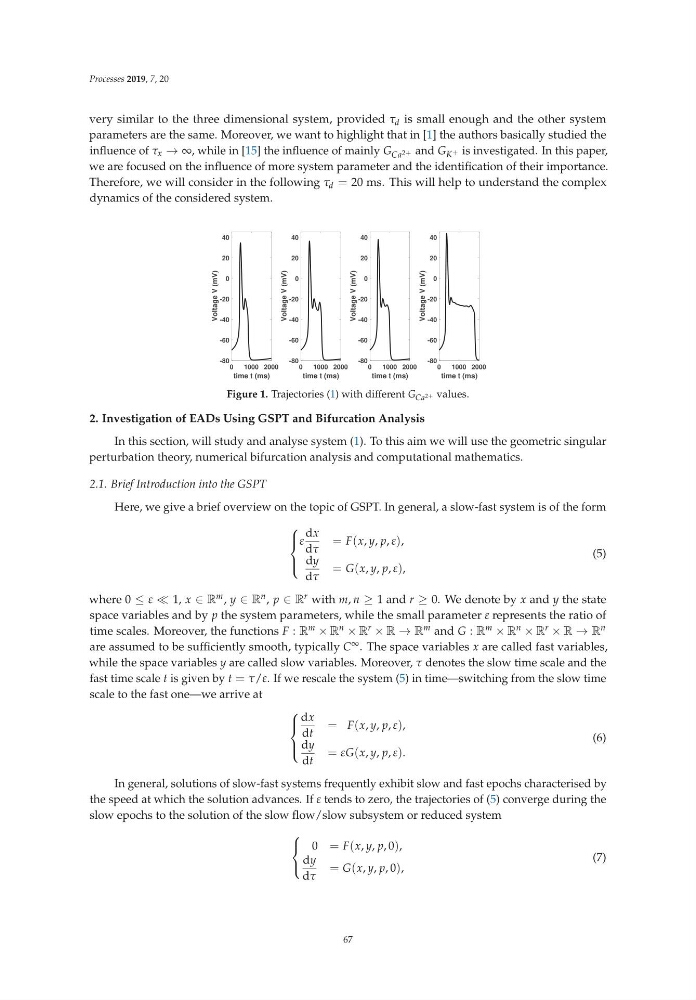
Therefore, we will consider in the following τ d = 20 ms. This will help to understand the complex
dynamics of the considered system.
0
1000 2000
time t (ms)
-80
-60
-40
-20
0
20
40
Voltage V (mV)
0
1000 2000
time t (ms)
-80
-60
-40
-20
0
20
40
Voltage V (mV)
0
1000 2000
time t (ms)
-80
-60
-40
-20
0
20
40
Voltage V (mV)
0
1000 2000
time t (ms)
-80
-60
-40
-20
0
20
40
Voltage V (mV)
Figure 1. Trajectories (1) with different G Ca 2+ values.
2. Investigation of EADs Using GSPT and Bifurcation Analysis
In this section, will study and analyse system (1). To this aim we will use the geometric singular
perturbation theory, numerical bifurcation analysis and computational mathematics.
2.1. Brief Introduction into the GSPT
Here, we give a brief overview on the topic of GSPT. In general, a slow-fast system is of the form
⎧
⎪
⎨
⎪
⎩
ε
dx
dτ
= F(x, y, p, ε),
dy
dτ
= G(x, y, p, ε),
(5)
where 0 ≤ ε ≪ 1, x ∈ R m , y ∈ R n , p ∈ R r with m, n ≥ 1 and r ≥ 0. We denote by x and y the state
space variables and by p the system parameters, while the small parameter ε represents the ratio of
time scales. Moreover, the functions F : R m × R n × R r × R → R m and G : R m × R n × R r × R → R n
are assumed to be sufficiently smooth, typically C ∞ . The space variables x are called fast variables,
while the space variables y are called slow variables. Moreover, τ denotes the slow time scale and the
fast time scale t is given by t = τ/ε. If we rescale the system (5) in time—switching from the slow time
scale to the fast one—we arrive at
⎧
⎪
⎨
⎪
⎩
dx
dt
= F(x, y, p, ε),
dy
dt
= εG(x, y, p, ε).
(6)
In general, solutions of slow-fast systems frequently exhibit slow and fast epochs characterised by
the speed at which the solution advances. If ε tends to zero, the trajectories of (5) converge during the
slow epochs to the solution of the slow flow/slow subsystem or reduced system
⎧
⎨
⎩
0 = F(x, y, p,0),
dy
dτ
= G(x, y, p,0),
(7)
67
very similar to the three dimensional system, provided τ d is small enough and the other system
parameters are the same. Moreover, we want to highlight that in [1] the authors basically studied the
influence of τ x → ∞, while in [15] the influence of mainly G Ca 2+ and G K + is investigated. In this paper,
we are focused on the influence of more system parameter and the identification of their importance.
Therefore, we will consider in the following τ d = 20 ms. This will help to understand the complex
dynamics of the considered system.
0
1000 2000
time t (ms)
-80
-60
-40
-20
0
20
40
Voltage V (mV)
0
1000 2000
time t (ms)
-80
-60
-40
-20
0
20
40
Voltage V (mV)
0
1000 2000
time t (ms)
-80
-60
-40
-20
0
20
40
Voltage V (mV)
0
1000 2000
time t (ms)
-80
-60
-40
-20
0
20
40
Voltage V (mV)
Figure 1. Trajectories (1) with different G Ca 2+ values.
2. Investigation of EADs Using GSPT and Bifurcation Analysis
In this section, will study and analyse system (1). To this aim we will use the geometric singular
perturbation theory, numerical bifurcation analysis and computational mathematics.
2.1. Brief Introduction into the GSPT
Here, we give a brief overview on the topic of GSPT. In general, a slow-fast system is of the form
⎧
⎪
⎨
⎪
⎩
ε
dx
dτ
= F(x, y, p, ε),
dy
dτ
= G(x, y, p, ε),
(5)
where 0 ≤ ε ≪ 1, x ∈ R m , y ∈ R n , p ∈ R r with m, n ≥ 1 and r ≥ 0. We denote by x and y the state
space variables and by p the system parameters, while the small parameter ε represents the ratio of
time scales. Moreover, the functions F : R m × R n × R r × R → R m and G : R m × R n × R r × R → R n
are assumed to be sufficiently smooth, typically C ∞ . The space variables x are called fast variables,
while the space variables y are called slow variables. Moreover, τ denotes the slow time scale and the
fast time scale t is given by t = τ/ε. If we rescale the system (5) in time—switching from the slow time
scale to the fast one—we arrive at
⎧
⎪
⎨
⎪
⎩
dx
dt
= F(x, y, p, ε),
dy
dt
= εG(x, y, p, ε).
(6)
In general, solutions of slow-fast systems frequently exhibit slow and fast epochs characterised by
the speed at which the solution advances. If ε tends to zero, the trajectories of (5) converge during the
slow epochs to the solution of the slow flow/slow subsystem or reduced system
⎧
⎨
⎩
0 = F(x, y, p,0),
dy
dτ
= G(x, y, p,0),
(7)
67