

Processes 2019, 7,20
⎧
⎪
⎪
⎪
⎪
⎪
⎨
⎪
⎪
⎪
⎪
⎪
⎩
folded saddle,
if λ 1,2 ∈ R and λ 1 λ 2 < 0,
folded saddle-node,
if λ 1,2 ∈ R and λ 1 λ 2 = 0,
folded node,
if λ 1,2 ∈ R and λ 1 λ 2 > 0,
folded focus,
if λ 1,2 ∈ C.
(11)
Here, we have to highlight that folded saddles, folded nodes and folded foci are also known
as canard points, see [22]. Even more, for sufficiently small values of the perturbation parameter ε
it is possible to calculate the maximal number of small oscillations of a MMO pattern, see [23,24].
For instance, if λ 1 and λ 2 are the eigenvalues of the linearisation of the desingularised system at a
folded node and μ = λ 1 /λ 2 with |λ 1 | < |λ 2 |, then the maximal number of small oscillations in the
MMO (in a neighbourhood of the folded node) is given by
s max :=
μ + 1
2μ
,
(12)
i.e., the greatest integer less than or equal to (μ + 1)/2μ, provided
√
ε ≪ μ.
2.2. The Study of EADs as MMOs
After this short introduction into the topic of GSPT, we will go on with the investigation of the
dynamics of our multiple time scale problem. To this aim we first have to derive a suitable model to
be able to apply this theory. To determine the different time scales we use a certain type of time scale
separation argument, cf. [25]. Thus, we introduce a new (dimensionless) time variable τ satisfying
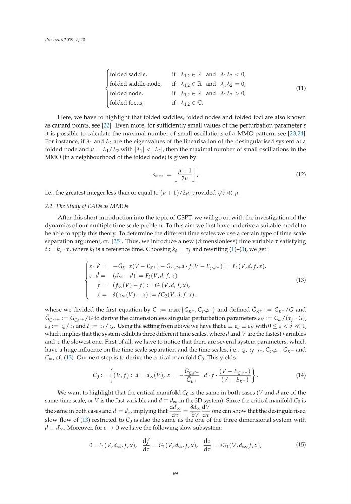
t := k t · τ, where k t is a reference time. Choosing k t = τ f and rewriting (1)–(3), we get:
⎧
⎪
⎪
⎪
⎪
⎪
⎨
⎪
⎪
⎪
⎪
⎪
⎩
ε · ˙
V = − ¯
G K + x(V − E K + ) − ¯
G Ca
2+ d · f (V − E Ca
2+ ) := F 1 (V, d, f , x),
ε · ˙
d =( d ∞ − d) := F 2 (V, d, f , x)
˙
f =( f ∞ (V) − f ) := G 1 (V, d, f , x),
˙
x = δ(x ∞ (V) − x) := δG 2 (V, d, f , x),
(13)
where we divided the first equation by G := max {G K + , G Ca 2+ } and defined ¯
G K + := G K + /G and
¯
G Ca 2+ := G Ca 2+ /G to derive the dimensionless singular perturbation parameters ε V := C m /(τ f · G),
ε d := τ d /τ f and δ := τ f /τ x . Using the setting from above we have that ε ≡ ε d ≡ ε V with 0 ≤ ε < δ ≪ 1,
which implies that the system exhibits three different time scales, where d and V are the fastest variables
and x the slowest one. First of all, we have to notice that there are several system parameters, which
have a huge influence on the time scale separation and the time scales, i.e., τ d , τ f , τ x , G Ca 2+ , G K + and
C m , cf. (13). Our next step is to derive the critical manifold C 0 . This yields
C 0 :=
(V, f ) : d = d ∞ (V), x = −
¯
G Ca 2+
¯
G K +
· d · f ·
(V − E Ca 2+ )
(V − E K + )
.
(14)
We want to highlight that the critical manifold C 0 is the same in both cases (V and d are of the
same time scale, or V is the fast variable and d ≡ d ∞ in the 3D system). Since the critical manifold C 0 is
the same in both cases and d = d ∞ implying that
dd ∞
dτ
=
∂d ∞
∂V
dV
dτ
one can show that the desingularised
slow flow of (13) restricted to C 0 is also the same as the one of the three dimensional system with
d ≡ d ∞ . Moreover, for ε → 0 we have the following slow subsystem:
0 =F 1 (V, d ∞ , f , x),
d f
dτ
= G 1 (V, d ∞ , f , x),
dx
dτ
= δG 1 (V, d ∞ , f , x),
(15)
69
⎧
⎪
⎪
⎪
⎪
⎪
⎨
⎪
⎪
⎪
⎪
⎪
⎩
folded saddle,
if λ 1,2 ∈ R and λ 1 λ 2 < 0,
folded saddle-node,
if λ 1,2 ∈ R and λ 1 λ 2 = 0,
folded node,
if λ 1,2 ∈ R and λ 1 λ 2 > 0,
folded focus,
if λ 1,2 ∈ C.
(11)
Here, we have to highlight that folded saddles, folded nodes and folded foci are also known
as canard points, see [22]. Even more, for sufficiently small values of the perturbation parameter ε
it is possible to calculate the maximal number of small oscillations of a MMO pattern, see [23,24].
For instance, if λ 1 and λ 2 are the eigenvalues of the linearisation of the desingularised system at a
folded node and μ = λ 1 /λ 2 with |λ 1 | < |λ 2 |, then the maximal number of small oscillations in the
MMO (in a neighbourhood of the folded node) is given by
s max :=
μ + 1
2μ
,
(12)
i.e., the greatest integer less than or equal to (μ + 1)/2μ, provided
√
ε ≪ μ.
2.2. The Study of EADs as MMOs
After this short introduction into the topic of GSPT, we will go on with the investigation of the
dynamics of our multiple time scale problem. To this aim we first have to derive a suitable model to
be able to apply this theory. To determine the different time scales we use a certain type of time scale
separation argument, cf. [25]. Thus, we introduce a new (dimensionless) time variable τ satisfying
t := k t · τ, where k t is a reference time. Choosing k t = τ f and rewriting (1)–(3), we get:
⎧
⎪
⎪
⎪
⎪
⎪
⎨
⎪
⎪
⎪
⎪
⎪
⎩
ε · ˙
V = − ¯
G K + x(V − E K + ) − ¯
G Ca
2+ d · f (V − E Ca
2+ ) := F 1 (V, d, f , x),
ε · ˙
d =( d ∞ − d) := F 2 (V, d, f , x)
˙
f =( f ∞ (V) − f ) := G 1 (V, d, f , x),
˙
x = δ(x ∞ (V) − x) := δG 2 (V, d, f , x),
(13)
where we divided the first equation by G := max {G K + , G Ca 2+ } and defined ¯
G K + := G K + /G and
¯
G Ca 2+ := G Ca 2+ /G to derive the dimensionless singular perturbation parameters ε V := C m /(τ f · G),
ε d := τ d /τ f and δ := τ f /τ x . Using the setting from above we have that ε ≡ ε d ≡ ε V with 0 ≤ ε < δ ≪ 1,
which implies that the system exhibits three different time scales, where d and V are the fastest variables
and x the slowest one. First of all, we have to notice that there are several system parameters, which
have a huge influence on the time scale separation and the time scales, i.e., τ d , τ f , τ x , G Ca 2+ , G K + and
C m , cf. (13). Our next step is to derive the critical manifold C 0 . This yields
C 0 :=
(V, f ) : d = d ∞ (V), x = −
¯
G Ca 2+
¯
G K +
· d · f ·
(V − E Ca 2+ )
(V − E K + )
.
(14)
We want to highlight that the critical manifold C 0 is the same in both cases (V and d are of the
same time scale, or V is the fast variable and d ≡ d ∞ in the 3D system). Since the critical manifold C 0 is
the same in both cases and d = d ∞ implying that
dd ∞
dτ
=
∂d ∞
∂V
dV
dτ
one can show that the desingularised
slow flow of (13) restricted to C 0 is also the same as the one of the three dimensional system with
d ≡ d ∞ . Moreover, for ε → 0 we have the following slow subsystem:
0 =F 1 (V, d ∞ , f , x),
d f
dτ
= G 1 (V, d ∞ , f , x),
dx
dτ
= δG 1 (V, d ∞ , f , x),
(15)
69