

Processes 2018, 6,39
2.1. Main Window (Figure 2)
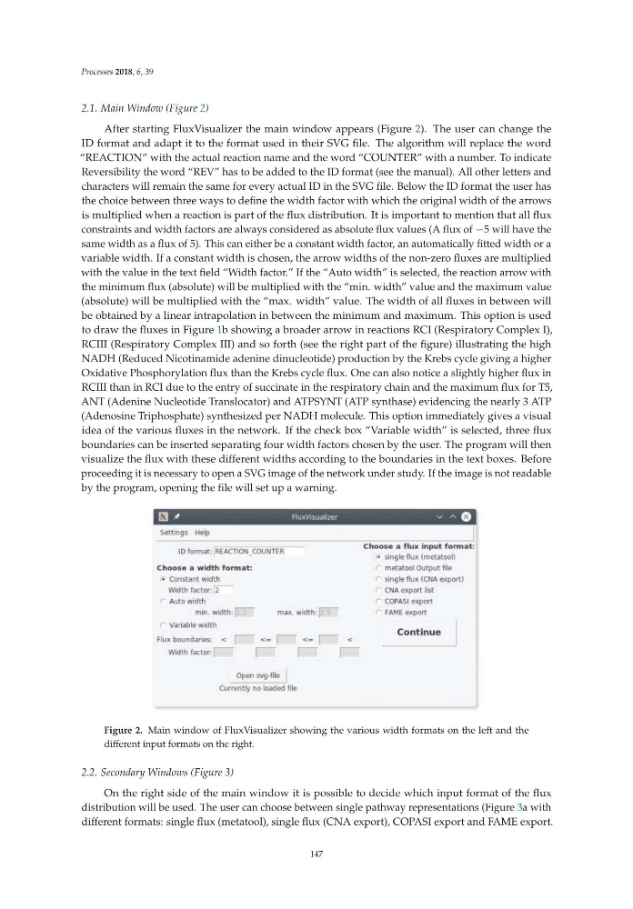
After starting FluxVisualizer the main window appears (Figure 2). The user can change the
ID format and adapt it to the format used in their SVG file. The algorithm will replace the word
“REACTION” with the actual reaction name and the word “COUNTER” with a number. To indicate
Reversibility the word “REV” has to be added to the ID format (see the manual). All other letters and
characters will remain the same for every actual ID in the SVG file. Below the ID format the user has
the choice between three ways to define the width factor with which the original width of the arrows
is multiplied when a reaction is part of the flux distribution. It is important to mention that all flux
constraints and width factors are always considered as absolute flux values (A flux of −5 will have the
same width as a flux of 5). This can either be a constant width factor, an automatically fitted width or a
variable width. If a constant width is chosen, the arrow widths of the non-zero fluxes are multiplied
with the value in the text field “Width factor.” If the “Auto width” is selected, the reaction arrow with
the minimum flux (absolute) will be multiplied with the “min. width” value and the maximum value
(absolute) will be multiplied with the “max. width” value. The width of all fluxes in between will
be obtained by a linear intrapolation in between the minimum and maximum. This option is used
to draw the fluxes in Figure 1b showing a broader arrow in reactions RCI (Respiratory Complex I),
RCIII (Respiratory Complex III) and so forth (see the right part of the figure) illustrating the high
NADH (Reduced Nicotinamide adenine dinucleotide) production by the Krebs cycle giving a higher
Oxidative Phosphorylation flux than the Krebs cycle flux. One can also notice a slightly higher flux in
RCIII than in RCI due to the entry of succinate in the respiratory chain and the maximum flux for T5,
ANT (Adenine Nucleotide Translocator) and ATPSYNT (ATP synthase) evidencing the nearly 3 ATP
(Adenosine Triphosphate) synthesized per NADH molecule. This option immediately gives a visual
idea of the various fluxes in the network. If the check box “Variable width” is selected, three flux
boundaries can be inserted separating four width factors chosen by the user. The program will then
visualize the flux with these different widths according to the boundaries in the text boxes. Before
proceeding it is necessary to open a SVG image of the network under study. If the image is not readable
by the program, opening the file will set up a warning.
Figure 2. Main window of FluxVisualizer showing the various width formats on the left and the
different input formats on the right.
2.2. Secondary Windows (Figure 3)
On the right side of the main window it is possible to decide which input format of the flux
distribution will be used. The user can choose between single pathway representations (Figure 3a with
different formats: single flux (metatool), single flux (CNA export), COPASI export and FAME export.
147
2.1. Main Window (Figure 2)
After starting FluxVisualizer the main window appears (Figure 2). The user can change the
ID format and adapt it to the format used in their SVG file. The algorithm will replace the word
“REACTION” with the actual reaction name and the word “COUNTER” with a number. To indicate
Reversibility the word “REV” has to be added to the ID format (see the manual). All other letters and
characters will remain the same for every actual ID in the SVG file. Below the ID format the user has
the choice between three ways to define the width factor with which the original width of the arrows
is multiplied when a reaction is part of the flux distribution. It is important to mention that all flux
constraints and width factors are always considered as absolute flux values (A flux of −5 will have the
same width as a flux of 5). This can either be a constant width factor, an automatically fitted width or a
variable width. If a constant width is chosen, the arrow widths of the non-zero fluxes are multiplied
with the value in the text field “Width factor.” If the “Auto width” is selected, the reaction arrow with
the minimum flux (absolute) will be multiplied with the “min. width” value and the maximum value
(absolute) will be multiplied with the “max. width” value. The width of all fluxes in between will
be obtained by a linear intrapolation in between the minimum and maximum. This option is used
to draw the fluxes in Figure 1b showing a broader arrow in reactions RCI (Respiratory Complex I),
RCIII (Respiratory Complex III) and so forth (see the right part of the figure) illustrating the high
NADH (Reduced Nicotinamide adenine dinucleotide) production by the Krebs cycle giving a higher
Oxidative Phosphorylation flux than the Krebs cycle flux. One can also notice a slightly higher flux in
RCIII than in RCI due to the entry of succinate in the respiratory chain and the maximum flux for T5,
ANT (Adenine Nucleotide Translocator) and ATPSYNT (ATP synthase) evidencing the nearly 3 ATP
(Adenosine Triphosphate) synthesized per NADH molecule. This option immediately gives a visual
idea of the various fluxes in the network. If the check box “Variable width” is selected, three flux
boundaries can be inserted separating four width factors chosen by the user. The program will then
visualize the flux with these different widths according to the boundaries in the text boxes. Before
proceeding it is necessary to open a SVG image of the network under study. If the image is not readable
by the program, opening the file will set up a warning.
Figure 2. Main window of FluxVisualizer showing the various width formats on the left and the
different input formats on the right.
2.2. Secondary Windows (Figure 3)
On the right side of the main window it is possible to decide which input format of the flux
distribution will be used. The user can choose between single pathway representations (Figure 3a with
different formats: single flux (metatool), single flux (CNA export), COPASI export and FAME export.
147