

500 ´ 500 pixel image. Each random SS stack was composed of 200 layers with a
scale increment of one. We note that the data required to conduct this normalization
procedure are an important reason (and limitation) for performing analysis on a
relatively small scene (500 ´ 500 pixels). For more in-depth information regarding
this normalization procedure see Hay et al. (2002a).
8.2.3.4 SS Blob Ranking and Vectors Once the lifetime of each SS blob is
defined, the binary blobs that correspond to a specific lifetime are used as a mask to
extract the integrated normalized (4D) volume (x, y, z, Lt n ) of each individual SS blob
from a normalized gray-level stack. These resulting normalized volumes are then
ranked from the highest to the lowest, and a user-determined number of significant SS
blobs are generated, from which the scale (t) representing the maximum 3D gray-level
blob volume (x, y, z) of each hyperblob is extracted. From these layers the associated
2D spatial support (i.e., binary blob) is identified, converted from a raster to a vector
polygon, and then related back to the corresponding structures in the image for further
examination (Figure 8.12). Thus, 4D SS blobs are simplified to 3D gray-level blobs,
which are further simplified to their 2D support region [i.e., modeled as a geographic
information system (GIS) polygon] and then to their corresponding real-world
structure in the original image. For a detailed nonmathematical description of SS
and blob feature detection, see Hay et al. (2002a).
8.3 DISCUSSION
8.3.1 Integrating Hierarch Theory and Scale Space
8.3.1.1 Integrating Hierarchy Theory to Reduce SS Processing Requirements
An important limitation of SS is that within an SS cube a significant amount of
“redundant” data result in large stack sizes. Based on the original gray-scale image
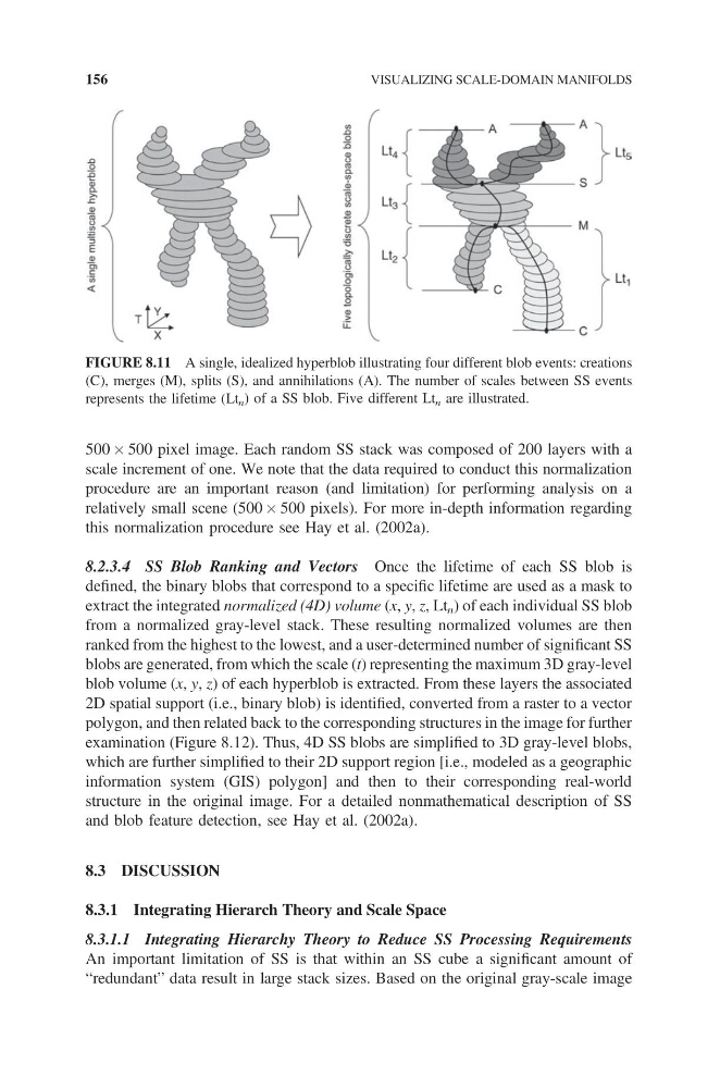
FIGURE 8.11 A single, idealized hyperblob illustrating four different blob events: creations
(C), merges (M), splits (S), and annihilations (A). The number of scales between SS events
represents the lifetime (Lt n ) of a SS blob. Five different Lt n are illustrated.
156
VISUALIZING SCALE-DOMAIN MANIFOLDS
scale increment of one. We note that the data required to conduct this normalization
procedure are an important reason (and limitation) for performing analysis on a
relatively small scene (500 ´ 500 pixels). For more in-depth information regarding
this normalization procedure see Hay et al. (2002a).
8.2.3.4 SS Blob Ranking and Vectors Once the lifetime of each SS blob is
defined, the binary blobs that correspond to a specific lifetime are used as a mask to
extract the integrated normalized (4D) volume (x, y, z, Lt n ) of each individual SS blob
from a normalized gray-level stack. These resulting normalized volumes are then
ranked from the highest to the lowest, and a user-determined number of significant SS
blobs are generated, from which the scale (t) representing the maximum 3D gray-level
blob volume (x, y, z) of each hyperblob is extracted. From these layers the associated
2D spatial support (i.e., binary blob) is identified, converted from a raster to a vector
polygon, and then related back to the corresponding structures in the image for further
examination (Figure 8.12). Thus, 4D SS blobs are simplified to 3D gray-level blobs,
which are further simplified to their 2D support region [i.e., modeled as a geographic
information system (GIS) polygon] and then to their corresponding real-world
structure in the original image. For a detailed nonmathematical description of SS
and blob feature detection, see Hay et al. (2002a).
8.3 DISCUSSION
8.3.1 Integrating Hierarch Theory and Scale Space
8.3.1.1 Integrating Hierarchy Theory to Reduce SS Processing Requirements
An important limitation of SS is that within an SS cube a significant amount of
“redundant” data result in large stack sizes. Based on the original gray-scale image
FIGURE 8.11 A single, idealized hyperblob illustrating four different blob events: creations
(C), merges (M), splits (S), and annihilations (A). The number of scales between SS events
represents the lifetime (Lt n ) of a SS blob. Five different Lt n are illustrated.
156
VISUALIZING SCALE-DOMAIN MANIFOLDS