

interval. “Best” values are defined as the most cloud free (highest VI values) pixels
with the closest to nadir view angle. Both the NDVI and enhanced vegetation index
(EVI) are available to end users, as well as several other derived products, including
LAI, net primary productivity, and other biophysical variables. Previous studies
(Nagler et al., 2005a,e) have shown that the EVI is significantly (p < 0.05) better
correlated with ground-measured ET than NDVI. Hence we used EVI to predict ET in
the Tamarix beetle studies. EVI is calculated from red, blue, and NIR bands as
described in Huete et al. (2002):
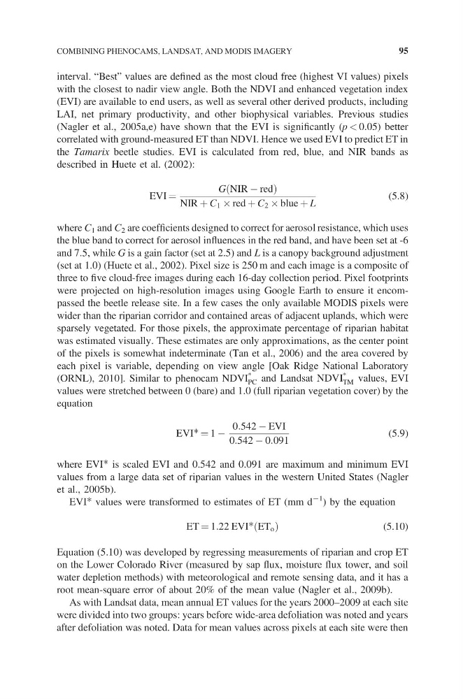
EVI =
G NIR − red
NIR + C 1 ´ red + C 2 ´ blue + L
(5.8)
where C 1 and C 2 are coefficients designed to correct for aerosol resistance, which uses
the blue band to correct for aerosol influences in the red band, and have been set at -6
and 7.5, while G is a gain factor (set at 2.5) and L is a canopy background adjustment
(set at 1.0) (Huete et al., 2002). Pixel size is 250 m and each image is a composite of
three to five cloud-free images during each 16-day collection period. Pixel footprints
were projected on high-resolution images using Google Earth to ensure it encompassed the beetle release site. In a few cases the only available MODIS pixels were
wider than the riparian corridor and contained areas of adjacent uplands, which were
sparsely vegetated. For those pixels, the approximate percentage of riparian habitat
was estimated visually. These estimates are only approximations, as the center point
of the pixels is somewhat indeterminate (Tan et al., 2006) and the area covered by
each pixel is variable, depending on view angle [Oak Ridge National Laboratory
(ORNL), 2010]. Similar to phenocam NDVI *
PC and Landsat NDVI *
TM values, EVI
values were stretched between 0 (bare) and 1.0 (full riparian vegetation cover) by the
equation
EVI* = 1 −
0:542 − EVI
0:542 − 0:091
(5.9)
where EVI* is scaled EVI and 0.542 and 0.091 are maximum and minimum EVI
values from a large data set of riparian values in the western United States (Nagler
et al., 2005b).
EVI* values were transformed to estimates of ET (mm d
−1
) by the equation
ET = 1:22 EVI* ET o
(5.10)
Equation (5.10) was developed by regressing measurements of riparian and crop ET
on the Lower Colorado River (measured by sap flux, moisture flux tower, and soil
water depletion methods) with meteorological and remote sensing data, and it has a
root mean-square error of about 20% of the mean value (Nagler et al., 2009b).
As with Landsat data, mean annual ET values for the years 2000–2009 at each site
were divided into two groups: years before wide-area defoliation was noted and years
after defoliation was noted. Data for mean values across pixels at each site were then
COMBINING PHENOCAMS, LANDSAT, AND MODIS IMAGERY
95
with the closest to nadir view angle. Both the NDVI and enhanced vegetation index
(EVI) are available to end users, as well as several other derived products, including
LAI, net primary productivity, and other biophysical variables. Previous studies
(Nagler et al., 2005a,e) have shown that the EVI is significantly (p < 0.05) better
correlated with ground-measured ET than NDVI. Hence we used EVI to predict ET in
the Tamarix beetle studies. EVI is calculated from red, blue, and NIR bands as
described in Huete et al. (2002):
EVI =
G NIR − red
NIR + C 1 ´ red + C 2 ´ blue + L
(5.8)
where C 1 and C 2 are coefficients designed to correct for aerosol resistance, which uses
the blue band to correct for aerosol influences in the red band, and have been set at -6
and 7.5, while G is a gain factor (set at 2.5) and L is a canopy background adjustment
(set at 1.0) (Huete et al., 2002). Pixel size is 250 m and each image is a composite of
three to five cloud-free images during each 16-day collection period. Pixel footprints
were projected on high-resolution images using Google Earth to ensure it encompassed the beetle release site. In a few cases the only available MODIS pixels were
wider than the riparian corridor and contained areas of adjacent uplands, which were
sparsely vegetated. For those pixels, the approximate percentage of riparian habitat
was estimated visually. These estimates are only approximations, as the center point
of the pixels is somewhat indeterminate (Tan et al., 2006) and the area covered by
each pixel is variable, depending on view angle [Oak Ridge National Laboratory
(ORNL), 2010]. Similar to phenocam NDVI *
PC and Landsat NDVI *
TM values, EVI
values were stretched between 0 (bare) and 1.0 (full riparian vegetation cover) by the
equation
EVI* = 1 −
0:542 − EVI
0:542 − 0:091
(5.9)
where EVI* is scaled EVI and 0.542 and 0.091 are maximum and minimum EVI
values from a large data set of riparian values in the western United States (Nagler
et al., 2005b).
EVI* values were transformed to estimates of ET (mm d
−1
) by the equation
ET = 1:22 EVI* ET o
(5.10)
Equation (5.10) was developed by regressing measurements of riparian and crop ET
on the Lower Colorado River (measured by sap flux, moisture flux tower, and soil
water depletion methods) with meteorological and remote sensing data, and it has a
root mean-square error of about 20% of the mean value (Nagler et al., 2009b).
As with Landsat data, mean annual ET values for the years 2000–2009 at each site
were divided into two groups: years before wide-area defoliation was noted and years
after defoliation was noted. Data for mean values across pixels at each site were then
COMBINING PHENOCAMS, LANDSAT, AND MODIS IMAGERY
95