

Conservation planning in a changing world
195
At local scales, within and among habitats within
regions ( ‘ sample areas ’ ), species accumulation is a
function of relative abundance distributions and beta
diversity (encompassing aspects of habitat heterogeneity and species turnover among sites). The z - values
typically observed for sample areas fall between 0.1
and 0.2. Across islands or disparate habitats within a
region (the ‘ archipelagic category ’ ), species richness
per island/habitat is affected by increased dispersal
limitation, due either to spatial distances between
similar habitat patches (e.g. islands in an archipelago)
or to ecological differences between habitats (e.g.
where frequency distributions of species differ greatly
across habitats within the region). The z - values typically observed for intra - provincial/archipelagic areas
fall between 0.25 and 0.55. At the largest scales, the
accumulation of species with increasing area is due to
the addition of species from separate biotic provinces
(the ‘ inter - provincial species – area relationship ’ ). The
z - values typically observed for inter - provincial areas
have a lower margin of z = 0.6 and range upwards,
with most lying around 0.9 – 1.0 or even higher (Table
8.1 ; Rosenzweig, 1995, 2001, 2004 ; Figure B8.1a ).
Rosenzweig ’ s work ( 1995 ; see also 2001, 2004 )
offered a more nuanced dynamic perception of the
SARs and the biological meaning of their slopes.
Fundamentally, the z is not just an indication of the
isolation of the system under study – a perception that
dominated the fi eld of island biogeography for more
than 40 years (Preston, 1962 ; MacArthur & Wilson,
1967 ) – but refl ects the dominant processes establishing species richness patterns. As Rosenzweig ( 1995 , p.
278) succinctly states: ‘ the slope of the species – area
curve refl ects the timescale that determines it ’ . These
timescales range from hours/days for curves from small
sample areas, to the millennia of evolutionary time
for the curves among different biotic provinces
(Box 8.1 ).
curve. Preston showed that a log – normal series of
abundance should give rise to a SAR with a slope ( z )
value of approximately 0.263 – towards the low end of
the range of values known at that time from islands and
above those of continental patches (for details see
Rosenzweig, 1995 , pp. 268 – 276). These differences
pointed to a role for isolation via population migration.
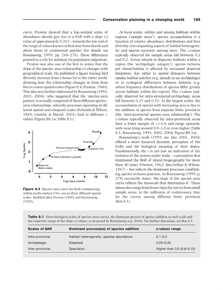
Preston was also one of the fi rst to notice that the
slope of the species – area relationship ( z ) changes with
geographical scale. He published a fi gure tracing bird
diversity increase from a house lot to the entire world,
showing how the relationship changes in form from
fi ne to coarse spatial scales (Figure 8.4 ; Preston, 1960 ).
This idea was further elaborated by Rosenzweig (1995,
2001, 2004) , who suggested that the ‘ species – area
pattern ’ is actually comprised of three different species –
area relationships, whereby processes operating at different spatial and temporal scales (Schmida & Wilson,
1985 ; Crawley & Harral, 2001 ) lead to different z -
values (Figure B8.1a ; Table 8.1 ).
Figure 8.4 Species – area curve for birds commencing
within north - eastern USA, across three different spatial
scales. Modifi ed after Preston (1960) and Rosenzweig
(1995) .
House lot,
Butler county
0
2
4
6
8
10
12
0
1
2
3
4
Preston Laboratory grounds
Western Pennsylvania
Eastern USA
Nearctic
World
Table 8.1 Three biological scales of species – area curves, the dominant process of species addition at each scale and
the respective range of the slope ( z ) values, as proposed by Rosenzweig (e.g. 2004 ). For further discussion, see Box 8.1 .
Scales of SAR
Dominant process(es) of species addition
z - values range
Intra - provincial
Habitat heterogeneity, species abundance
0.1 – 0.2
Archipelagic
Dispersal
0.25 – 0.45
Inter - provincial
Speciation
Higher than 0.6 (0.8 – 0.10)
195
At local scales, within and among habitats within
regions ( ‘ sample areas ’ ), species accumulation is a
function of relative abundance distributions and beta
diversity (encompassing aspects of habitat heterogeneity and species turnover among sites). The z - values
typically observed for sample areas fall between 0.1
and 0.2. Across islands or disparate habitats within a
region (the ‘ archipelagic category ’ ), species richness
per island/habitat is affected by increased dispersal
limitation, due either to spatial distances between
similar habitat patches (e.g. islands in an archipelago)
or to ecological differences between habitats (e.g.
where frequency distributions of species differ greatly
across habitats within the region). The z - values typically observed for intra - provincial/archipelagic areas
fall between 0.25 and 0.55. At the largest scales, the
accumulation of species with increasing area is due to
the addition of species from separate biotic provinces
(the ‘ inter - provincial species – area relationship ’ ). The
z - values typically observed for inter - provincial areas
have a lower margin of z = 0.6 and range upwards,
with most lying around 0.9 – 1.0 or even higher (Table
8.1 ; Rosenzweig, 1995, 2001, 2004 ; Figure B8.1a ).
Rosenzweig ’ s work ( 1995 ; see also 2001, 2004 )
offered a more nuanced dynamic perception of the
SARs and the biological meaning of their slopes.
Fundamentally, the z is not just an indication of the
isolation of the system under study – a perception that
dominated the fi eld of island biogeography for more
than 40 years (Preston, 1962 ; MacArthur & Wilson,
1967 ) – but refl ects the dominant processes establishing species richness patterns. As Rosenzweig ( 1995 , p.
278) succinctly states: ‘ the slope of the species – area
curve refl ects the timescale that determines it ’ . These
timescales range from hours/days for curves from small
sample areas, to the millennia of evolutionary time
for the curves among different biotic provinces
(Box 8.1 ).
curve. Preston showed that a log – normal series of
abundance should give rise to a SAR with a slope ( z )
value of approximately 0.263 – towards the low end of
the range of values known at that time from islands and
above those of continental patches (for details see
Rosenzweig, 1995 , pp. 268 – 276). These differences
pointed to a role for isolation via population migration.
Preston was also one of the fi rst to notice that the
slope of the species – area relationship ( z ) changes with
geographical scale. He published a fi gure tracing bird
diversity increase from a house lot to the entire world,
showing how the relationship changes in form from
fi ne to coarse spatial scales (Figure 8.4 ; Preston, 1960 ).
This idea was further elaborated by Rosenzweig (1995,
2001, 2004) , who suggested that the ‘ species – area
pattern ’ is actually comprised of three different species –
area relationships, whereby processes operating at different spatial and temporal scales (Schmida & Wilson,
1985 ; Crawley & Harral, 2001 ) lead to different z -
values (Figure B8.1a ; Table 8.1 ).
Figure 8.4 Species – area curve for birds commencing
within north - eastern USA, across three different spatial
scales. Modifi ed after Preston (1960) and Rosenzweig
(1995) .
House lot,
Butler county
0
2
4
6
8
10
12
0
1
2
3
4
Preston Laboratory grounds
Western Pennsylvania
Eastern USA
Nearctic
World
Table 8.1 Three biological scales of species – area curves, the dominant process of species addition at each scale and
the respective range of the slope ( z ) values, as proposed by Rosenzweig (e.g. 2004 ). For further discussion, see Box 8.1 .
Scales of SAR
Dominant process(es) of species addition
z - values range
Intra - provincial
Habitat heterogeneity, species abundance
0.1 – 0.2
Archipelagic
Dispersal
0.25 – 0.45
Inter - provincial
Speciation
Higher than 0.6 (0.8 – 0.10)