

Continental Shelf Research 232 (2022) 104629
4
Gradient filter (Sobel, 1990) as follows:
k(x, y) =
1
2πσ 2 exp
−(x
2 + y
2 )
2π 2
(1)
where, k (x,y) is the matrix of the kernel used to convolute the original
image; x and y are the pixel’s position along the abscissa and ordinate
axes respectively. σ
2
is the variance of the 3x3 pixel matrix.
The horizontal and vertical components of the Sobel gradient (Eq. (2)
and Eq. (3), respectively) were separately computed and combined into
the final gradient (Eq. (4)):
G h [x][y] = k(x, y) *
⎧
⎨
⎩
−1 −2 −1
0
0
0
1
2
1
⎫
⎬
⎭
(2)
G v [x][y] = k(x, y) *
⎧
⎨
⎩
−1 0 1
−2 0 2
−1 0 1
⎫
⎬
⎭
(3)
Sobel G [x][y] =
̅̅̅̅̅̅̅̅̅̅̅̅̅̅̅̅̅̅̅̅̅̅̅̅̅̅̅̅̅̅̅̅̅̅̅̅̅̅
G
2
h [x][y] + G
2
v [x][y]
√
(4)
As spurious gradients are mainly associated with atmospheric perturbations in the vicinity of clouds, a maximum threshold value of the
local Sobel gradient of Chl-a was considered to detect outlier pixels
(Fig. 3a), at a maximum distance of 5 km from cloud borders (black
areas in Fig. 3b). After several tests, two thresholds were defined: 0.4 mg
m
-3
km
-1
and 1 mg m
-3
km
-1
respectively for the coastal zone (distance
from the coast <5 km) (Fig. 3c) and the offshore area.
2.3.2. Temporal variability (TV) criteria
Each daily individual Chl-a pixel value of a given day (Day0) was
compared to the average value of the previous day (Day-1) and the
following day (Day+1) when one or both values are available to detect
anomalous Chl-a variations through time, as given by Eq. (5):
TV = Day 0 −
(
Day −1 + Day +1
2
)
(5)
This difference was then compared with the maximum threshold of
temporal variability set at 2 mg m
-3
. Furthermore, this test was applied
in the offshore domain only (distance from coast >20 km) to consider
the higher spatio-temporal variability of the coastal environment
(Fig. 3e).
2.3.3. Isolated pixel (IP) removal
This criterion is used to eliminate pixels closely associated with a
cloud structure. We considered that Chl-a pixels bordered by more than
five cloudy pixels (including those isolated in a cloud) belong to the
same atmospheric structure and should be eliminated (Fig. 3f).
2.3.4. Combination of criteria
The three criteria mentioned above were cumulated, and the pixels
marked by at least one criterion were removed. The resulting daily data
are significantly less noisy, as shown in Fig. 3h. A fortnightly climatology of Chl-a at 1-km resolution is then computed for the whole AB.
2.4. Comparison between in-situ and satellite Chl-a data
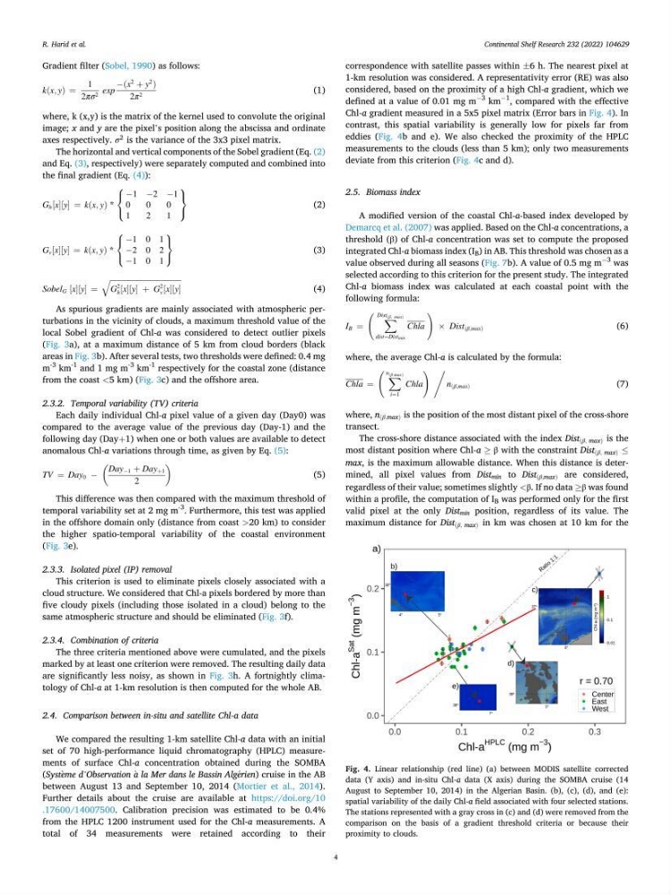
We compared the resulting 1-km satellite Chl-a data with an initial
set of 70 high-performance liquid chromatography (HPLC) measurements of surface Chl-a concentration obtained during the SOMBA
(Syst` eme d’Observation `
a la Mer dans le Bassin Alg´ erien) cruise in the AB
between August 13 and September 10, 2014 (Mortier et al., 2014).
Further details about the cruise are available at https://doi.org/10
.17600/14007500. Calibration precision was estimated to be 0.4%
from the HPLC 1200 instrument used for the Chl-a measurements. A
total of 34 measurements were retained according to their
correspondence with satellite passes within ±6 h. The nearest pixel at
1-km resolution was considered. A representativity error (RE) was also
considered, based on the proximity of a high Chl-a gradient, which we
defined at a value of 0.01 mg m
−3
km
−1
, compared with the effective
Chl-a gradient measured in a 5x5 pixel matrix (Error bars in Fig. 4). In
contrast, this spatial variability is generally low for pixels far from
eddies (Fig. 4b and e). We also checked the proximity of the HPLC
measurements to the clouds (less than 5 km); only two measurements
deviate from this criterion (Fig. 4c and d).
2.5. Biomass index
A modified version of the coastal Chl-a-based index developed by
Demarcq et al. (2007) was applied. Based on the Chl-a concentrations, a
threshold (β) of Chl-a concentration was set to compute the proposed
integrated Chl-a biomass index (I B ) in AB. This threshold was chosen as a
value observed during all seasons (Fig. 7b). A value of 0.5 mg m
−3
was
selected according to this criterion for the present study. The integrated
Chl-a biomass index was calculated at each coastal point with the
following formula:
I B =
(
∑
Dist (β, max)
dist=Distmin
Chla
)
× Dist (β,max)
(6)
where, the average Chl-a is calculated by the formula:
Chla =
(
∑
n (β,max)
i=1
Chla
) /
n (β,max)
(7)
where, n (β,max) is the position of the most distant pixel of the cross-shore
transect.
The cross-shore distance associated with the index Dist (β, max) is the
most distant position where Chl-a ≥ β with the constraint Dist (β, max) ≤
max, is the maximum allowable distance. When this distance is determined, all pixel values from Dist min to Dist (β,max) are considered,
regardless of their value; sometimes slightly <β. If no data ≥β was found
within a profile, the computation of I B was performed only for the first
valid pixel at the only Dist min position, regardless of its value. The
maximum distance for Dist (β, max) in km was chosen at 10 km for the
Fig. 4. Linear relationship (red line) (a) between MODIS satellite corrected
data (Y axis) and in-situ Chl-a data (X axis) during the SOMBA cruise (14
August to September 10, 2014) in the Algerian Basin. (b), (c), (d), and (e):
spatial variability of the daily Chl-a field associated with four selected stations.
The stations represented with a gray cross in (c) and (d) were removed from the
comparison on the basis of a gradient threshold criteria or because their
proximity to clouds.
R. Harid et al.
4
Gradient filter (Sobel, 1990) as follows:
k(x, y) =
1
2πσ 2 exp
−(x
2 + y
2 )
2π 2
(1)
where, k (x,y) is the matrix of the kernel used to convolute the original
image; x and y are the pixel’s position along the abscissa and ordinate
axes respectively. σ
2
is the variance of the 3x3 pixel matrix.
The horizontal and vertical components of the Sobel gradient (Eq. (2)
and Eq. (3), respectively) were separately computed and combined into
the final gradient (Eq. (4)):
G h [x][y] = k(x, y) *
⎧
⎨
⎩
−1 −2 −1
0
0
0
1
2
1
⎫
⎬
⎭
(2)
G v [x][y] = k(x, y) *
⎧
⎨
⎩
−1 0 1
−2 0 2
−1 0 1
⎫
⎬
⎭
(3)
Sobel G [x][y] =
̅̅̅̅̅̅̅̅̅̅̅̅̅̅̅̅̅̅̅̅̅̅̅̅̅̅̅̅̅̅̅̅̅̅̅̅̅̅
G
2
h [x][y] + G
2
v [x][y]
√
(4)
As spurious gradients are mainly associated with atmospheric perturbations in the vicinity of clouds, a maximum threshold value of the
local Sobel gradient of Chl-a was considered to detect outlier pixels
(Fig. 3a), at a maximum distance of 5 km from cloud borders (black
areas in Fig. 3b). After several tests, two thresholds were defined: 0.4 mg
m
-3
km
-1
and 1 mg m
-3
km
-1
respectively for the coastal zone (distance
from the coast <5 km) (Fig. 3c) and the offshore area.
2.3.2. Temporal variability (TV) criteria
Each daily individual Chl-a pixel value of a given day (Day0) was
compared to the average value of the previous day (Day-1) and the
following day (Day+1) when one or both values are available to detect
anomalous Chl-a variations through time, as given by Eq. (5):
TV = Day 0 −
(
Day −1 + Day +1
2
)
(5)
This difference was then compared with the maximum threshold of
temporal variability set at 2 mg m
-3
. Furthermore, this test was applied
in the offshore domain only (distance from coast >20 km) to consider
the higher spatio-temporal variability of the coastal environment
(Fig. 3e).
2.3.3. Isolated pixel (IP) removal
This criterion is used to eliminate pixels closely associated with a
cloud structure. We considered that Chl-a pixels bordered by more than
five cloudy pixels (including those isolated in a cloud) belong to the
same atmospheric structure and should be eliminated (Fig. 3f).
2.3.4. Combination of criteria
The three criteria mentioned above were cumulated, and the pixels
marked by at least one criterion were removed. The resulting daily data
are significantly less noisy, as shown in Fig. 3h. A fortnightly climatology of Chl-a at 1-km resolution is then computed for the whole AB.
2.4. Comparison between in-situ and satellite Chl-a data
We compared the resulting 1-km satellite Chl-a data with an initial
set of 70 high-performance liquid chromatography (HPLC) measurements of surface Chl-a concentration obtained during the SOMBA
(Syst` eme d’Observation `
a la Mer dans le Bassin Alg´ erien) cruise in the AB
between August 13 and September 10, 2014 (Mortier et al., 2014).
Further details about the cruise are available at https://doi.org/10
.17600/14007500. Calibration precision was estimated to be 0.4%
from the HPLC 1200 instrument used for the Chl-a measurements. A
total of 34 measurements were retained according to their
correspondence with satellite passes within ±6 h. The nearest pixel at
1-km resolution was considered. A representativity error (RE) was also
considered, based on the proximity of a high Chl-a gradient, which we
defined at a value of 0.01 mg m
−3
km
−1
, compared with the effective
Chl-a gradient measured in a 5x5 pixel matrix (Error bars in Fig. 4). In
contrast, this spatial variability is generally low for pixels far from
eddies (Fig. 4b and e). We also checked the proximity of the HPLC
measurements to the clouds (less than 5 km); only two measurements
deviate from this criterion (Fig. 4c and d).
2.5. Biomass index
A modified version of the coastal Chl-a-based index developed by
Demarcq et al. (2007) was applied. Based on the Chl-a concentrations, a
threshold (β) of Chl-a concentration was set to compute the proposed
integrated Chl-a biomass index (I B ) in AB. This threshold was chosen as a
value observed during all seasons (Fig. 7b). A value of 0.5 mg m
−3
was
selected according to this criterion for the present study. The integrated
Chl-a biomass index was calculated at each coastal point with the
following formula:
I B =
(
∑
Dist (β, max)
dist=Distmin
Chla
)
× Dist (β,max)
(6)
where, the average Chl-a is calculated by the formula:
Chla =
(
∑
n (β,max)
i=1
Chla
) /
n (β,max)
(7)
where, n (β,max) is the position of the most distant pixel of the cross-shore
transect.
The cross-shore distance associated with the index Dist (β, max) is the
most distant position where Chl-a ≥ β with the constraint Dist (β, max) ≤
max, is the maximum allowable distance. When this distance is determined, all pixel values from Dist min to Dist (β,max) are considered,
regardless of their value; sometimes slightly <β. If no data ≥β was found
within a profile, the computation of I B was performed only for the first
valid pixel at the only Dist min position, regardless of its value. The
maximum distance for Dist (β, max) in km was chosen at 10 km for the
Fig. 4. Linear relationship (red line) (a) between MODIS satellite corrected
data (Y axis) and in-situ Chl-a data (X axis) during the SOMBA cruise (14
August to September 10, 2014) in the Algerian Basin. (b), (c), (d), and (e):
spatial variability of the daily Chl-a field associated with four selected stations.
The stations represented with a gray cross in (c) and (d) were removed from the
comparison on the basis of a gradient threshold criteria or because their
proximity to clouds.
R. Harid et al.