

Continental Shelf Research 232 (2022) 104629
5
coastal area and 80 km for the next offshore area, according to the
average structure of the cross-profiles (Fig. 6b). It is important to note
that for continuity reasons, the first (inner) pixel of the offshore area was
considered the pixel immediately offshore of the last of the coastal areas.
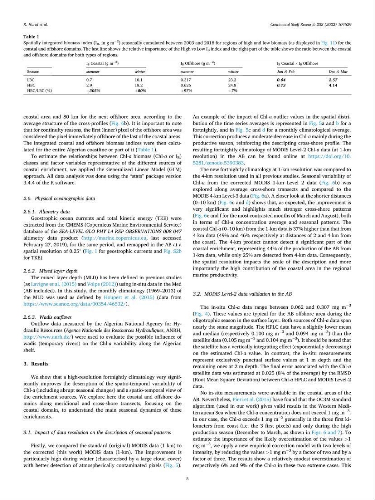
The integrated coastal and offshore biomass indices were then calculated for the entire Algerian coastline or part of it (Table 1).
To estimate the relationships between Chl-a biomass (Chl-a or I B )
classes and factor variables representative of the different sources of
coastal enrichment, we applied the Generalized Linear Model (GLM)
approach. All data analysis was done using the “stats” package version
3.4.4 of the R software.
2.6. Physical oceanographic data
2.6.1. Altimetry data
Geostrophic ocean currents and total kinetic energy (TKE) were
extracted from the CMEMS (Copernicus Marine Environmental Service)
database of the SEA-LEVEL GLO PHY L4 REP OBSERVATIONS 008 047
altimetry data product (http://marine.copernicus.eu, last accessed
February 27, 2019), for the same period, and remapped in the AB at a
spatial resolution of 0.25
◦
(Fig. 1 for geostrophic currents and Fig. S2b
for TKE).
2.6.2. Mixed layer depth
The mixed layer depth (MLD) has been defined in previous studies
(as Lavigne et al. (2015) and Volpe (2012)) using in-situ data in the Med
(AB included). In this study, the monthly climatology (1969–2013) of
the MLD was used as defined by Houpert et al. (2015) (data from
https://www.seanoe.org/data/00354/46532/).
2.6.3. Wadis outflows
Outflow data measured by the Algerian National Agency for Hydraulic Resources (Agence Nationale des Ressources Hydrauliques, ANRH,
http://www.anrh.dz/) were used to evaluate the possible influence of
wadis (temporary rivers) on the Chl-a variability along the Algerian
shelf.
3. Results
We show that a high-resolution fortnightly climatology very significantly improves the description of the spatio-temporal variability of
Chl-a (including abrupt seasonal changes) and a spatio-temporal view of
the enrichment sources. We explore here the coastal and offshore domains along meridional and cross-shore transects, focusing on the
coastal domain, to understand the main seasonal dynamics of these
enrichments.
3.1. Impact of data resolution on the description of seasonal patterns
Firstly, we compared the standard (original) MODIS data (1-km) to
the corrected (this work) MODIS data (1-km). The improvement is
particularly high during winter (characterised by a large cloud cover)
with better detection of atmospherically contaminated pixels (Fig. 5).
An example of the impact of Chl-a outlier values in the spatial distribution of the time series averages is represented in Fig. 5a and b for a
fortnightly, and in Fig. 5c and d for a monthly climatological average.
This correction produces a moderate decrease in Chl-a mainly during the
productive season, reinforcing the descripting cross-shore profile. The
resulting fortnightly climatology of MODIS Level-2 Chl-a data (at 1-km
resolution) in the AB can be found online at https://doi.org/10.
5281/zenodo.5390383.
The new fortnightly climatology at 1-km resolution was compared to
the 4-km resolution used in all previous studies. Seasonal variability of
Chl-a from the corrected MODIS 1-km Level 2 data (Fig. 6b) was
explored along average cross-shore transects and compared to the
MODIS 4-km Level-3 data (Fig. 6a). A closer look at the shorter distances
(0–10 km) (Fig. 6c and d) shows that, as expected, the improvement is
very significant and highlights much stronger cross-shore patterns
(Fig. 6e and f for the most contrasted months of March and August), both
in terms of Chl-a concentration average and seasonal patterns. The
coastal Chl-a (0–10 km) from the 1-km data is 37% higher than that from
4-km data (49% and 46% respectively at distances of 2 and 4-km from
the coast). The 4-km product cannot detect a significant part of the
coastal enrichment, representing 44% of the production of the AB from
1-km data, while only 25% are detected from 4-km data. Consequently,
the spatial resolution impacts the scale of the description and more
importantly the high contribution of the coastal area in the regional
marine productivity.
3.2. MODIS Level-2 data validation in the AB
The in-situ Chl-a data range between 0.062 and 0.307 mg m
−3
(Fig. 4). These values are typical for the AB offshore area during the
oligotrophic season in the surface layer. Both sources of Chl-a data span
nearly the same magnitude. The HPLC data have a slightly lower mean
and median (respectively 0.100 mg m
−3
and 0.094 mg m
−3
) than the
satellite data (0.105 mg m
−3
and 0.104 mg m
−3
). It should be noted that
the satellite has a vertically integrating effect (exponentially decreasing)
on the estimated Chl-a value. In contrast, the in-situ measurements
represent exclusively punctual surface values at 1 m depth and the
remaining ones at 2 m depth. The final error associated with the Chl-a
satellite data was estimated at 0.025 (8% of the average) by the RMSD
(Root Mean Square Deviation) between Chl-a HPLC and MODIS Level-2
data.
No in-situ measurements were available in the coastal areas of the
AB. Nevertheless, Pieri et al. (2015) have found that the OC3M standard
algorithm (used in our work) gives valid results in the Western Mediterranean Sea when the Chl-a concentration does not exceed 1 mg m
−3
.
In our case, the Chl-a exceeds 1 mg m
−3
generally in the three first kilometers from coast (i.e. the 3 first pixels) and only during the high
production season (December to March, as shown in Figs. 6 and 7). To
estimate the importance of the likely overestimation of the values >1
mg m
−3
, we apply a new empirical correction model with two levels of
intensity, by reducing the values >1 mg m
−3
by a factor of two and by a
factor of three. The results show a relatively modest overestimation of
respectively 6% and 9% of the Chl-a in these two extreme cases. This
Table 1
Spatially integrated biomass index (I B , in g m
−2
) seasonally cumulated between 2003 and 2018 for regions of high and low biomass (as displayed in Fig. 11) for the
coastal and offshore domains. The last line shows the relative importance of the High vs Low I B index and the right part of the table shows the ratio between the coastal
and offshore domains for both types of regions.
I B Coastal (g m
−2
)
I B Offshore (g m
−2
)
I B Coastal / I B Offshore
Season
summer
winter
summer
winter
Jan & Feb
Dec & Mar
LBC
0.7
10.1
0.317
23.2
0.64
2.57
HBC
2.9
18.2
0.626
24.8
0.73
4.14
HBC/LBC (%)
+305%
+80%
+97%
+7%
R. Harid et al.
5
coastal area and 80 km for the next offshore area, according to the
average structure of the cross-profiles (Fig. 6b). It is important to note
that for continuity reasons, the first (inner) pixel of the offshore area was
considered the pixel immediately offshore of the last of the coastal areas.
The integrated coastal and offshore biomass indices were then calculated for the entire Algerian coastline or part of it (Table 1).
To estimate the relationships between Chl-a biomass (Chl-a or I B )
classes and factor variables representative of the different sources of
coastal enrichment, we applied the Generalized Linear Model (GLM)
approach. All data analysis was done using the “stats” package version
3.4.4 of the R software.
2.6. Physical oceanographic data
2.6.1. Altimetry data
Geostrophic ocean currents and total kinetic energy (TKE) were
extracted from the CMEMS (Copernicus Marine Environmental Service)
database of the SEA-LEVEL GLO PHY L4 REP OBSERVATIONS 008 047
altimetry data product (http://marine.copernicus.eu, last accessed
February 27, 2019), for the same period, and remapped in the AB at a
spatial resolution of 0.25
◦
(Fig. 1 for geostrophic currents and Fig. S2b
for TKE).
2.6.2. Mixed layer depth
The mixed layer depth (MLD) has been defined in previous studies
(as Lavigne et al. (2015) and Volpe (2012)) using in-situ data in the Med
(AB included). In this study, the monthly climatology (1969–2013) of
the MLD was used as defined by Houpert et al. (2015) (data from
https://www.seanoe.org/data/00354/46532/).
2.6.3. Wadis outflows
Outflow data measured by the Algerian National Agency for Hydraulic Resources (Agence Nationale des Ressources Hydrauliques, ANRH,
http://www.anrh.dz/) were used to evaluate the possible influence of
wadis (temporary rivers) on the Chl-a variability along the Algerian
shelf.
3. Results
We show that a high-resolution fortnightly climatology very significantly improves the description of the spatio-temporal variability of
Chl-a (including abrupt seasonal changes) and a spatio-temporal view of
the enrichment sources. We explore here the coastal and offshore domains along meridional and cross-shore transects, focusing on the
coastal domain, to understand the main seasonal dynamics of these
enrichments.
3.1. Impact of data resolution on the description of seasonal patterns
Firstly, we compared the standard (original) MODIS data (1-km) to
the corrected (this work) MODIS data (1-km). The improvement is
particularly high during winter (characterised by a large cloud cover)
with better detection of atmospherically contaminated pixels (Fig. 5).
An example of the impact of Chl-a outlier values in the spatial distribution of the time series averages is represented in Fig. 5a and b for a
fortnightly, and in Fig. 5c and d for a monthly climatological average.
This correction produces a moderate decrease in Chl-a mainly during the
productive season, reinforcing the descripting cross-shore profile. The
resulting fortnightly climatology of MODIS Level-2 Chl-a data (at 1-km
resolution) in the AB can be found online at https://doi.org/10.
5281/zenodo.5390383.
The new fortnightly climatology at 1-km resolution was compared to
the 4-km resolution used in all previous studies. Seasonal variability of
Chl-a from the corrected MODIS 1-km Level 2 data (Fig. 6b) was
explored along average cross-shore transects and compared to the
MODIS 4-km Level-3 data (Fig. 6a). A closer look at the shorter distances
(0–10 km) (Fig. 6c and d) shows that, as expected, the improvement is
very significant and highlights much stronger cross-shore patterns
(Fig. 6e and f for the most contrasted months of March and August), both
in terms of Chl-a concentration average and seasonal patterns. The
coastal Chl-a (0–10 km) from the 1-km data is 37% higher than that from
4-km data (49% and 46% respectively at distances of 2 and 4-km from
the coast). The 4-km product cannot detect a significant part of the
coastal enrichment, representing 44% of the production of the AB from
1-km data, while only 25% are detected from 4-km data. Consequently,
the spatial resolution impacts the scale of the description and more
importantly the high contribution of the coastal area in the regional
marine productivity.
3.2. MODIS Level-2 data validation in the AB
The in-situ Chl-a data range between 0.062 and 0.307 mg m
−3
(Fig. 4). These values are typical for the AB offshore area during the
oligotrophic season in the surface layer. Both sources of Chl-a data span
nearly the same magnitude. The HPLC data have a slightly lower mean
and median (respectively 0.100 mg m
−3
and 0.094 mg m
−3
) than the
satellite data (0.105 mg m
−3
and 0.104 mg m
−3
). It should be noted that
the satellite has a vertically integrating effect (exponentially decreasing)
on the estimated Chl-a value. In contrast, the in-situ measurements
represent exclusively punctual surface values at 1 m depth and the
remaining ones at 2 m depth. The final error associated with the Chl-a
satellite data was estimated at 0.025 (8% of the average) by the RMSD
(Root Mean Square Deviation) between Chl-a HPLC and MODIS Level-2
data.
No in-situ measurements were available in the coastal areas of the
AB. Nevertheless, Pieri et al. (2015) have found that the OC3M standard
algorithm (used in our work) gives valid results in the Western Mediterranean Sea when the Chl-a concentration does not exceed 1 mg m
−3
.
In our case, the Chl-a exceeds 1 mg m
−3
generally in the three first kilometers from coast (i.e. the 3 first pixels) and only during the high
production season (December to March, as shown in Figs. 6 and 7). To
estimate the importance of the likely overestimation of the values >1
mg m
−3
, we apply a new empirical correction model with two levels of
intensity, by reducing the values >1 mg m
−3
by a factor of two and by a
factor of three. The results show a relatively modest overestimation of
respectively 6% and 9% of the Chl-a in these two extreme cases. This
Table 1
Spatially integrated biomass index (I B , in g m
−2
) seasonally cumulated between 2003 and 2018 for regions of high and low biomass (as displayed in Fig. 11) for the
coastal and offshore domains. The last line shows the relative importance of the High vs Low I B index and the right part of the table shows the ratio between the coastal
and offshore domains for both types of regions.
I B Coastal (g m
−2
)
I B Offshore (g m
−2
)
I B Coastal / I B Offshore
Season
summer
winter
summer
winter
Jan & Feb
Dec & Mar
LBC
0.7
10.1
0.317
23.2
0.64
2.57
HBC
2.9
18.2
0.626
24.8
0.73
4.14
HBC/LBC (%)
+305%
+80%
+97%
+7%
R. Harid et al.