

105
9 Photoautotrophic Productivity in Eutrophic Ecosystems
Similarly, annual production (ΣΣP) can be predicted from
chl-a concentration, light attenuation coefficient ( k w ) and the
chl-a specific extinction coefficient ( η) using an equation developed by Vollenweider (Clasen and Bernhardt 1980)
(9.5)
A more intensive discussion of depth-time integrated production calculation and associated models can be found in
Rodhe (1965) and Vollenweider (1965a, b, 1970).
Kimmel et al. (1990) provided a detailed table of the magnitude and variability of ΣA in reservoirs of different trophy.
On an annual basis, phytoplankton production is not significantly different from phytoplankton production in natural
lakes (Brylinsky 1980; Wetzel 2001, p. 386 ff.). Daily productivity in most reservoirs, however, is likely more variable
than in most natural lakes. About 30–40 % of the lakes and
reservoirs included in these references are eutrophic. This
is certainly an underestimation because most of the waters
worldwide are small and shallow with plenty of light and
nutrients (Downing et al. 2006; Downing 2010). This group
therefore should be among the most productive systems of
the world (Lewis 2011). Similarly, productivity of large rivers is likely to rise owing to increasing eutrophication (Dokulil 2012). Global change will further enhance freshwater
eutrophication (Dokulil and Teubner 2011).
[g C m
−2 y
−1
] = K
Chl − a
k w + η × Chl − a
9.5 Defining Trophic Boundary Conditions
Trophic boundaries were commonly deduced from column
integrated rates per square metre of lake surface (mg m
−2
)
either per day or per year.
Boundaries defined for integral daily rates by HendersonSellers and Markland (1987) in Table 9.1 are not very different from those by Schönborn (2003). Trophic levels were
expanded to cover hypertrophic conditions by Håkanson and
Boulion (2001).
Their ranges of average annual production (Table 9.2) are
much lower for the trophic categories than those stated by
Schönborn 2003 (Table 9.1).
Håkanson and Boulion (2001) then further added an ultra-oligotrophic level basing trophic classification on fixed
steps of mean summer chl-a using a factor of 10 (Table 9.3)
which was also used earlier by Håkanson and Peters (1995;
Table 9.3) in their modelling approach.
Limits by Wetzel (2001) are higher particularly for eutrophic conditions. In addition, his system expands the trophic
categories by adding ultra-oligotrophic and dystrophic levels
(Table 9.4)
Klapper (1992) and Felföldy (1987) considerably expanded and refined trophic categories to be able to better
differentiate lakes in regions where waters are primarily at
higher trophic level (Tables 9.4 and 9.5).
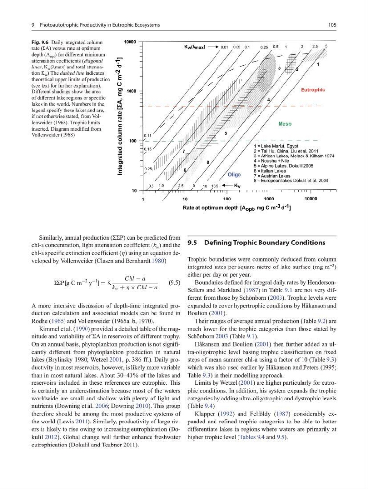
Fig. 9.6 Daily integrated column
rate (ΣA) versus rate at optimum
depth (A opt ) for different minimum
attenuation coefficients ( diagonal
lines, K w (λmax) and total attenuation K w ) The dashed line indicates
theoretical upper limits of production
(see text for further explanation).
Different shadings show the area
of different lake regions or specific
lakes in the world. Numbers in the
legend specify these lakes and are,
if not otherwise stated, from Vollenweider (1968). Trophic limits
inserted. Diagram modified from
Vollenweider (1968)
9 Photoautotrophic Productivity in Eutrophic Ecosystems
Similarly, annual production (ΣΣP) can be predicted from
chl-a concentration, light attenuation coefficient ( k w ) and the
chl-a specific extinction coefficient ( η) using an equation developed by Vollenweider (Clasen and Bernhardt 1980)
(9.5)
A more intensive discussion of depth-time integrated production calculation and associated models can be found in
Rodhe (1965) and Vollenweider (1965a, b, 1970).
Kimmel et al. (1990) provided a detailed table of the magnitude and variability of ΣA in reservoirs of different trophy.
On an annual basis, phytoplankton production is not significantly different from phytoplankton production in natural
lakes (Brylinsky 1980; Wetzel 2001, p. 386 ff.). Daily productivity in most reservoirs, however, is likely more variable
than in most natural lakes. About 30–40 % of the lakes and
reservoirs included in these references are eutrophic. This
is certainly an underestimation because most of the waters
worldwide are small and shallow with plenty of light and
nutrients (Downing et al. 2006; Downing 2010). This group
therefore should be among the most productive systems of
the world (Lewis 2011). Similarly, productivity of large rivers is likely to rise owing to increasing eutrophication (Dokulil 2012). Global change will further enhance freshwater
eutrophication (Dokulil and Teubner 2011).
[g C m
−2 y
−1
] = K
Chl − a
k w + η × Chl − a
9.5 Defining Trophic Boundary Conditions
Trophic boundaries were commonly deduced from column
integrated rates per square metre of lake surface (mg m
−2
)
either per day or per year.
Boundaries defined for integral daily rates by HendersonSellers and Markland (1987) in Table 9.1 are not very different from those by Schönborn (2003). Trophic levels were
expanded to cover hypertrophic conditions by Håkanson and
Boulion (2001).
Their ranges of average annual production (Table 9.2) are
much lower for the trophic categories than those stated by
Schönborn 2003 (Table 9.1).
Håkanson and Boulion (2001) then further added an ultra-oligotrophic level basing trophic classification on fixed
steps of mean summer chl-a using a factor of 10 (Table 9.3)
which was also used earlier by Håkanson and Peters (1995;
Table 9.3) in their modelling approach.
Limits by Wetzel (2001) are higher particularly for eutrophic conditions. In addition, his system expands the trophic
categories by adding ultra-oligotrophic and dystrophic levels
(Table 9.4)
Klapper (1992) and Felföldy (1987) considerably expanded and refined trophic categories to be able to better
differentiate lakes in regions where waters are primarily at
higher trophic level (Tables 9.4 and 9.5).
Fig. 9.6 Daily integrated column
rate (ΣA) versus rate at optimum
depth (A opt ) for different minimum
attenuation coefficients ( diagonal
lines, K w (λmax) and total attenuation K w ) The dashed line indicates
theoretical upper limits of production
(see text for further explanation).
Different shadings show the area
of different lake regions or specific
lakes in the world. Numbers in the
legend specify these lakes and are,
if not otherwise stated, from Vollenweider (1968). Trophic limits
inserted. Diagram modified from
Vollenweider (1968)