

200
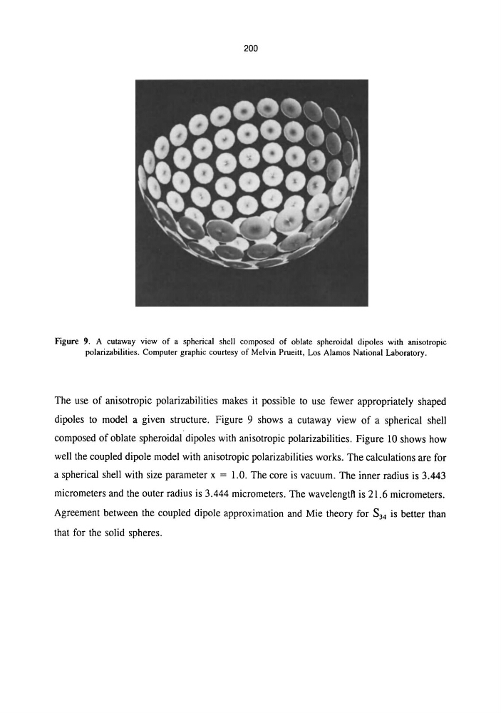
Figure 9. A cutaway view of a spherical shell composed of oblate spheroidal dipoles with anisotropic
polarizabilities. Computer graphic courtesy of Melvin Prueitt, Los Alamos National Laboratory.
The use of anisotropic polarizabilities makes it possible to use fewer appropriately shaped
dipoles to model a given structure. Figure 9 shows a cutaway view of a spherical shell
composed of oblate spheroidal dipoles with anisotropic polarizabilities. Figure 10 shows how
well the coupled dipole model with anisotropic polarizabilities works. The calculations are for
a spherical shell with size parameter x = 1.0. The core is vacuum. The inner radius is 3.443
micrometers and the outer radius is 3.444 micrometers. The wavelengtll is 21.6 micrometers.
Agreement between the coupled dipole approximation and Mie theory for S34 is better than
that for the solid spheres.
Figure 9. A cutaway view of a spherical shell composed of oblate spheroidal dipoles with anisotropic
polarizabilities. Computer graphic courtesy of Melvin Prueitt, Los Alamos National Laboratory.
The use of anisotropic polarizabilities makes it possible to use fewer appropriately shaped
dipoles to model a given structure. Figure 9 shows a cutaway view of a spherical shell
composed of oblate spheroidal dipoles with anisotropic polarizabilities. Figure 10 shows how
well the coupled dipole model with anisotropic polarizabilities works. The calculations are for
a spherical shell with size parameter x = 1.0. The core is vacuum. The inner radius is 3.443
micrometers and the outer radius is 3.444 micrometers. The wavelengtll is 21.6 micrometers.
Agreement between the coupled dipole approximation and Mie theory for S34 is better than
that for the solid spheres.