

198
SPHERE x
1.5
0
- 6
-
-2
'"
I
a
I
S
\
o -4
-
X 4
X -6
~
~
-8
2
~-10
U)
U) -12
"'-.
0
0
30
60
90
120
150
180
30
60
90
120
150
180
ANGLE (degrees)
ANGLE (degrees)
7
10
-
6
- 5
~
d
I
C
I
0
5
0
0
-
4
- ~
x
2S -5
1
~
3
\
-10
OJ
~ -15
/
OJ
1
~
,
U)
U)
0
-20
-.-/
-1
-25
0
30
60
90
120
150
180
0
30
60
90
120
150
180
ANGLE (degrees)
ANGLE (degrees)
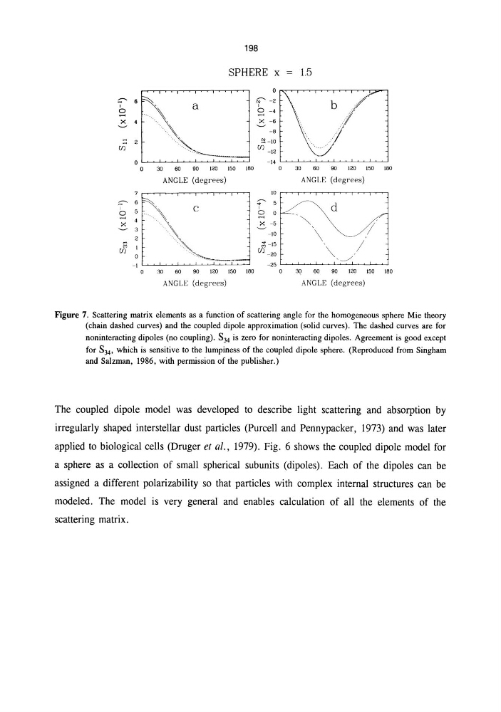
Figure 7. Scattering matrix elements as a function of scattering angle for the homogeneous sphere Mie theory
(chain dashed curves) and the coupled dipole approximation (solid curves). The dashed curves are for
noninteracting dipoles (no coupling). S34 is zero for noninteracting dipoles. Agreement is good except
for S34. which is sensitive to the lumpiness of the coupled dipole sphere. (Reproduced from Singham
and Salzman, 1986, with permission of the publisher.)
The coupled dipole model was developed to describe light scattering and absorption by
irregularly shaped interstellar dust particles (Purcell and Pennypacker, 1973) and was later
applied to biological cells (Druger et al., 1979). Fig. 6 shows the coupled dipole model for
a sphere as a collection of small spherical subunits (dipoles). Each of the dipoles can be
assigned a different polarizability so that particles with complex internal structures can be
modeled. The model is very general and enables calculation of all the elements of the
scattering matrix.
SPHERE x
1.5
0
- 6
-
-2
'"
I
a
I
S
\
o -4
-
X 4
X -6
~
~
-8
2
~-10
U)
U) -12
"'-.
0
0
30
60
90
120
150
180
30
60
90
120
150
180
ANGLE (degrees)
ANGLE (degrees)
7
10
-
6
- 5
~
d
I
C
I
0
5
0
0
-
4
- ~
x
2S -5
1
~
3
\
-10
OJ
~ -15
/
OJ
1
~
,
U)
U)
0
-20
-.-/
-1
-25
0
30
60
90
120
150
180
0
30
60
90
120
150
180
ANGLE (degrees)
ANGLE (degrees)
Figure 7. Scattering matrix elements as a function of scattering angle for the homogeneous sphere Mie theory
(chain dashed curves) and the coupled dipole approximation (solid curves). The dashed curves are for
noninteracting dipoles (no coupling). S34 is zero for noninteracting dipoles. Agreement is good except
for S34. which is sensitive to the lumpiness of the coupled dipole sphere. (Reproduced from Singham
and Salzman, 1986, with permission of the publisher.)
The coupled dipole model was developed to describe light scattering and absorption by
irregularly shaped interstellar dust particles (Purcell and Pennypacker, 1973) and was later
applied to biological cells (Druger et al., 1979). Fig. 6 shows the coupled dipole model for
a sphere as a collection of small spherical subunits (dipoles). Each of the dipoles can be
assigned a different polarizability so that particles with complex internal structures can be
modeled. The model is very general and enables calculation of all the elements of the
scattering matrix.