

304
12: Teerasit Kasetkasem, Pramod K. Varshney
Fig. 12.15. Color composite of hyperspectral image (2.04660 Ilm, 1.16690 Ilm, and
0.64910 Ilm) acquired by the HyMap sensor. For a colored version of this figure, see the
end of the book
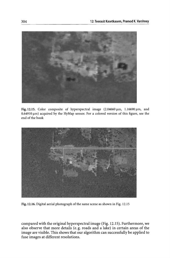
Fig. 12.16. Digital aerial photograph of the same scene as shown in Fig. 12.15
compared with the original hyperspectral image (Fig. 12.15). Furthermore, we
also observe that more details (e. g. roads and a lake) in certain areas of the
image are visible. This shows that our algorithm can successfully be applied to
fuse images at different resolutions.
12: Teerasit Kasetkasem, Pramod K. Varshney
Fig. 12.15. Color composite of hyperspectral image (2.04660 Ilm, 1.16690 Ilm, and
0.64910 Ilm) acquired by the HyMap sensor. For a colored version of this figure, see the
end of the book
Fig. 12.16. Digital aerial photograph of the same scene as shown in Fig. 12.15
compared with the original hyperspectral image (Fig. 12.15). Furthermore, we
also observe that more details (e. g. roads and a lake) in certain areas of the
image are visible. This shows that our algorithm can successfully be applied to
fuse images at different resolutions.