

260
11: Teerasit Kasetkasem, Manoj K. Arora, Pramod K. Varshney
i. e.,
Pr(X) = A exp [- L V d X)]
CeT
(11.2)
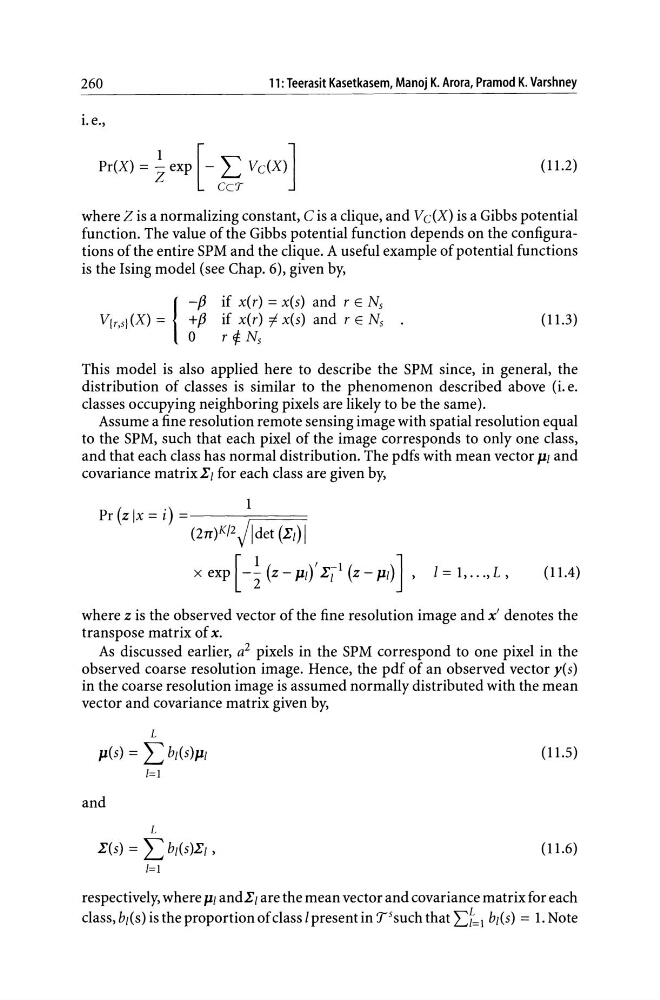
where Z is a normalizing constant, C is a clique, and V dX) is a Gibbs potential
function. The value of the Gibbs potential function depends on the configurations of the entire SPM and the clique. A useful example of potential functions
is the Ising model (see Chap. 6), given by,
1 - f3 if x(r) = x(s) and r E Ns
V{r,sj(X) =
+f3 if x(r) "x(s) and r E Ns
o r 4- Ns
(l1.3)
This model is also applied here to describe the SPM since, in general, the
distribution of classes is similar to the phenomenon described above (i. e.
classes occupying neighboring pixels are likely to be the same).
Assume a fine resolution remote sensing image with spatial resolution equal
to the SPM, such that each pixel of the image corresponds to only one class,
and that each class has normal distribution. The pdfs with mean vector PI and
covariance matrix II for each class are given by,
Pr(zlx=i)
1
(2rr)K/2 Jldet (II) I
x exp [ -~ (z - PI)' III (z - PI) ] ' 1 = 1, .. . ,L, (11.4)
where z is the observed vector of the fine resolution image and x' denotes the
transpose matrix of x.
As discussed earlier, a 2 pixels in the SPM correspond to one pixel in the
observed coarse resolution image. Hence, the pdf of an observed vector y(s)
in the coarse resolution image is assumed normally distributed with the mean
vector and covariance matrix given by,
L
p(s) = L bz(S)PI
(l1.5)
1=1
and
L
I(s) = L bl(s)II ,
(l1.6)
1=1
respectively, where PI andII are the mean vector and covariance matrix for each
class, bz(s) is the proportion of class 1 present in TSsuch that L::T=l bl(s) = 1. Note
11: Teerasit Kasetkasem, Manoj K. Arora, Pramod K. Varshney
i. e.,
Pr(X) = A exp [- L V d X)]
CeT
(11.2)
where Z is a normalizing constant, C is a clique, and V dX) is a Gibbs potential
function. The value of the Gibbs potential function depends on the configurations of the entire SPM and the clique. A useful example of potential functions
is the Ising model (see Chap. 6), given by,
1 - f3 if x(r) = x(s) and r E Ns
V{r,sj(X) =
+f3 if x(r) "x(s) and r E Ns
o r 4- Ns
(l1.3)
This model is also applied here to describe the SPM since, in general, the
distribution of classes is similar to the phenomenon described above (i. e.
classes occupying neighboring pixels are likely to be the same).
Assume a fine resolution remote sensing image with spatial resolution equal
to the SPM, such that each pixel of the image corresponds to only one class,
and that each class has normal distribution. The pdfs with mean vector PI and
covariance matrix II for each class are given by,
Pr(zlx=i)
1
(2rr)K/2 Jldet (II) I
x exp [ -~ (z - PI)' III (z - PI) ] ' 1 = 1, .. . ,L, (11.4)
where z is the observed vector of the fine resolution image and x' denotes the
transpose matrix of x.
As discussed earlier, a 2 pixels in the SPM correspond to one pixel in the
observed coarse resolution image. Hence, the pdf of an observed vector y(s)
in the coarse resolution image is assumed normally distributed with the mean
vector and covariance matrix given by,
L
p(s) = L bz(S)PI
(l1.5)
1=1
and
L
I(s) = L bl(s)II ,
(l1.6)
1=1
respectively, where PI andII are the mean vector and covariance matrix for each
class, bz(s) is the proportion of class 1 present in TSsuch that L::T=l bl(s) = 1. Note